Laboratory work in informatics. Excel Labs

Ministry of Education and Science

Russian Federation

Federal State Autonomous Educational Institution

higher professional education

National Research Nuclear University MEPhI

Volgodonsk Engineering and Technology Institute - branch of NRNU MEPhI

Creating tables

METHODOLOGICAL INSTRUCTIONSto laboratory work

in computer science in the programmicrosoftexcel

Volgodonsk 2010

UDC 519.683(076.5)

Reviewer tech. Sciences Z.O. Kavrishvili

Compiler V.A. Mace

Creating tables. Guidelines for laboratory work in MicrosortExcel. 2010. 13 p.

The guidelines contain explanations and recommendations for performing laboratory work on the computer science course in the MicrosortExcel program.

_____________________________________________________________________________

ã Volgodonsk Institute of National Research Nuclear University MEPhI, 2010

ã Bulava V.A., 2010

Laboratory work

Creating tables in the programexcelby automating data entry.

Goal of the work. To consolidate the acquired knowledge of creating, editing and formatting tables in Excel.

Formulation of the problem.

Compute function value y = f(x)/ g(x) for all X on the interval [ a, b] step by step To. Meaning of functions f(x) , g(x) , the value of the ends of the interval a And b and step value To is given from table 1 in the Appendix according to the option for a particular specialty.

The solution must be obtained in the form of tables "Main" and "Auxiliary".

Computed function values at copy to column TO without formulas .

The Excel program is launched using the commands Start → Programs →microsortexcel.

When creating a table, merge cells A1:H1 in the first row and place the text "Tables" in the center.

In the second line, merge cells A2: E2 and place the text "Main" in the center. Merge cells G2:H2 and center the text "Auxiliary"

In cell A3, enter the text "No. p / p". In cells B3:F3, place the names of the columns, respectively: X ; f(x)=…( according to your choice) ; g(x)=…( according to your choice) ; y= f(x)/ g(x).

In cells G3:H3, place the names of the columns accordingly: a ; To.

When autofilling the data of the main table in formulas, use absolute, relative and mixed addressing of cells.

In the "Main" and "Auxiliary" tables, the contents of the cells must be aligned to the center of the cell, and have a font size of 12 pt.

The font color of the table titles should be blue.

Color the outer borders of the tables blue, the internal borders green, and the cell fill yellow.

Reporting Form.

Provide the result of the laboratory work in the form of a report in printed or electronic form.

The printed version of the report must contain:

a) title page

b) the purpose of the work;

c) setting the task;

d) the result of the task.

2. Provide the result of the laboratory work in electronic form on a 3.5-inch diskette as a file with the name "Tables".

Control questions.

What is absolute, relative, mixed addressing?

How does autofill cells with numbers, formulas?

What are the ways to align the contents of a cell?

How can I change the color and thickness of the lines of the outer and inner borders of the table?

How can I change the background color of table cells?

Typical example.

Calculate the value of the function y \u003d x ∙ sin (x) / (x + 1) on the segment with a step of 0.1. The solution is presented in the form of a table. Computed function values at copy to column TO without formulas .

Solution.

In this case f(x) = x∙ sin(x) , g(x) = x+1 , a =0 , b = 2 , k = 0.1

1. In the first row of the table, select cells A1:H1. Execute the command Format → Cells, in the window that opens, expand the tab alignment and choose the item cell merging. In the center of the merged cells, enter the text "Tables".

2. Similarly, in the second row, merge cells A2: E2 and place the text “Main” in the center and merge cells G2: H2, and place the text “Auxiliary” in the center.

3. In the third line in cell A3, enter the text No. p / p ( name of the first column of the table ) , in cell B3 - X(name of the second column of the table ), cell C3 - f(x)= x∙ sin(x) , in cell D3 - g(x)= x+1 , in cell E3 - y=f(x)/ g(x) , in cell G3 - a, in cell H3 - k.

4. In cell A4, enter 1 and fill in cells A5:A24 with numbers from 2 to 21. To do this, select cell A4 (make it current), it will be highlighted in a black frame. Hover the mouse cursor over the fill marker (black cross in the lower right corner of the cell) and by pressing the right mouse button drag the fill marker along the column A so that the black frame covers cells A5:A24. Releasing the right mouse button, in the menu that opens, select the item fill. Cells A5: A24 will be filled with numbers 2; 3; 4 ...

5. In cell G4, enter the value 0 (value of the left end of the interval).

6. In cell H4, enter the value 0,1 (step size).

7. Fill in the column IN values X:

In cell B4, enter the formula =$ G$4 (initial value of x), the $ sign indicates absolute addressing. In cell B5, enter the formula =B4+$H$4. This means that the initial value of x will be increased by the step value;

using the autocomplete method, fill in cells B5:B24 with this formula. Select cell B5. Hover the mouse pointer over the fill handle and click left mouse button, drag the fill handle so that the black frame covers cells B5:B24. Column B will be filled with numbers 0; 0.1; 0,2;…, and the corresponding formulas will be in the formula bar.

8. Fill in the C column with the values of the function f(x)=x∙sin(x). In cell C4, enter the formula =B4∙sin(B4). Let's fill cells C5:C24 with this formula using the autocomplete method.

9. Fill in column D with the values of the function g(x)=x+1. In cell D4, enter the formula =B4+1. Let's fill cells D5:D24 with this formula using the autocomplete method.

10. Fill in column E with the values of the function y=f(x)/g(x). In cell E4, enter the formula =C4/D4, fill cells E5:E24 with this formula using the autocomplete method.

11. Let's frame the tables:

12. Change the background color of the cells of the main and auxiliary tables:

select the main table;

enter menu commands Format → Cells → View. In the window that opens, select the color yellow. Let's click on the OK button.

select the auxiliary table and change the background color of the cells in the same way.

13. In the main table, the values obtained as a result of calculations at copy to column TO without formulas:

select cells E4:E24;

move the mouse pointer over the outline of the black frame so that it takes the form of an arrow;

by pressing the right mouse button and without releasing it, move the mouse pointer to cell K4;

releasing the right mouse button, in the context menu that opens, select the item copy only values.

As a result of the work, we get the following tables:


Main						Auxiliary

Application

Table 1



	x 2 – 1+ cos 2 (x)
	3 - x-sin 2 (x)

	12x - 3- lg 2 (x)
	5x + 6cos 2 (x)


	5x - x 3 - cos 2 (x)
		3 + x 2 cos 2 (x)
	3 + x 3 - tg 2 (x)
	4x 2 - 9- lg 2 (x)

	2 cos 2 (x)+ 5
		cos2 (x) + x2

	2x2-sin2(x)
	4x 3 - cos 2 (x)
	3ln 2 (x) + x 2

	3sin(x) – x 3	4 + x + cos 2 (x)
	4x 3 -sin 2 (x)
	5x 2 + lg 2 (x)
	2x 3 - x 2 + 7	4 cos 2 (x) + x 2
	3x 2 – 5x cos 2 (x)
	2sin(x) – x 2



	3cos(x) + tg(x)


	5 + x 3 -4 lg 2 (x)
	4x3 – 2x2-7	5 cos 2(x) + 4x

Application

Table 1 continued

Task for students of the specialty
	f(x)	g(x)

	3x -sin 2(x)
		1 + x 2 cos 2 (x)
	12x - 3 cos 2 (x)



	5x - x 2 + 3
		5 + x 2 + 10x



	2cos 2(x) + 5x


	2x2-sin(x)
	9x3 - cos(x2)
	5sin 2 (x) + x 3

	3sin(x) – x 3
	3x2-sin(x3)

	8x3-x2+1

	2sin 2 (x 2) - x

	4cos(x 3) - 3x





	4x3 - 2x2 + 7

SAMARA STATE ACADEMY OF COMMUNICATIONS

Department of Informatics

COMPUTER SCIENCE

Spreadsheet MS Excel

Guidelines for performing laboratory work

for students of the specialty OPU of all forms of education

Compiled by: Makarova I.S.

Ermolenko T.I.

Samara 2006

Computer science. Spreadsheet MS Excel. [Text]: methodological instructions for performing laboratory work for students of the specialty of the OP of all forms of education. - Part 2 / compilers: I.S. Makarova, T.I. Ermolenko. - Samara: SamGAPS, 2006. - 44 p.

Approved at the meeting of the Department of Informatics on 04/06/2006, protocol No. 8.

Published by decision of the editorial and publishing council of the academy.

These guidelines are practical guide on mastering the techniques of working in a popular spreadsheet processor Microsoft Excel. The main elements of the interface, techniques and technologies for working with data necessary for creating tables, performing calculations and constructing diagrams are considered. Additional features of MS Excel, such as working with text functions, mathematical calculations, data analysis, are considered. To master the work in a spreadsheet will help the implementation of the proposed practical tasks, which contain detailed step by step instructions to get the final result.

The use of these guidelines assumes that students know the basics of working with operating sheath Windows.

Editor: E.A. Krasnova

Computer layout: R.R. Abrahamyan

Signed for publication on 15.06.06. Format 60x90 1/16.

Writing paper. The print is operational. Conv. p.l. 2.75.

Circulation 200 copies. Order No. 118.

Introduction

Microsoft Excel is quite powerful and easy to use electronic spreadsheet processor, designed to solve a wide range of planning and economic, accounting and statistical, scientific, technical, mathematical and other problems. MS Excel is based on working with spreadsheets.

A spreadsheet consists of rows and columns, at the intersection of which cells are located, and in this sense it is analogous to an ordinary table. But unlike an ordinary one, a spreadsheet serves not only for visual representation, but also for processing numerical, textual and graphic information stored in computer memory. Excel can operate on table cells in the same way that programming languages operate on variables.

Excel supports file formats marked with the xl* extension, and native Excel documents are located in files with the xls extension.

Excel has a built-in help system that provides the user with detailed description features of the package and offers demo examples to better understand the basic principles of their use.

Laboratory work №1. Basics of working with MS Excel

Goal of the work: get acquainted with the basic elements of a spreadsheet processor, methods for entering information into tables, formatting techniques

When starting MS Excel ( Start/Programs/Microsoft Excel ) a spreadsheet window appears on the screen with a document loaded into it, which is called the Workbook (Fig. 1):

Rice. 1. MS Excel window

Window Excel programs contains all the standard elements inherent in a Windows application window:

program icon

title line;

menu bar

toolbars;

Status bar

scrollbars.

The Excel menu bar differs from the Word menu bar with the command Data (instead of Table ). The toolbar has special buttons for numerical data - monetary and percentage formats; thousands separator; increasing and decreasing the bit depth of a number; button to merge and center text in a group of cells.

Below the toolbar is Formula bar, which is used to enter and edit data in cells. On the left side of the formula bar is a drop-down list − Name field, which displays the address of the current cell. In the same line, when entering formulas, three buttons appear to control the input process.

At the intersection of the column with row numbers and the row with the designation of the columns, there is a button Select all, which is used to select the entire worksheet.

Below the working field is a line with worksheet labels.

Consider basic concepts of MS Excel.

The Excel document is called workbook, it consists of a collection worksheets. By default, each workbook contains 3 worksheets, but their number can be changed from 1 to 255. The worksheet has a tabular structure and consists of 65,536 rows and 256 columns. Rows are numbered, and columns are denoted by Latin letters. alphabets A,B,C, …, Z,AA, AB,AC,…,BA, BB,…,IV.

active sheet(current sheet) of a workbook is the sheet that the user is currently working on. The active sheet tab always has a lighter background color with its name displayed in bold. By clicking on the labels, you can move from one sheet to another within the workbook. To move through the workbook sheets, you can also use the key combinations: Ctrl + Page Down and Ctrl + Page Up or a group of four buttons located in the lower left corner of the Excel working window.

At the intersection of a row and a column is cell- the smallest structural unit of the worksheet. Each cell has address, which is formed from the name of the column and the number of the row at the intersection of which it is located. Thus, the address of cell C7 means that this cell is located at the intersection of column C and row 7 of the current worksheet. In cases where it is necessary to refer to cells located on other worksheets, the name of the worksheet on which they are located is indicated before the address (for example, Sheet4!G9).

Active cell(current) is the cell in which the mouse cursor is located, which has the shape of a rectangular frame. You can enter data into the active cell and perform various operations on it.

Link- a way to specify the address of the cell. Cell references are used as arguments in formulas and functions. When performing calculations, the value in the cell to which the link points is inserted in the place of the link.

Cell Block(range) - represents a rectangular area of adjacent cells. A block of cells can consist of a single cell, a row (or part of it), a column (or part of it), or a sequence of rows or columns (or parts of them). Block address is a combination of the addresses of the upper left and lower right cells of the block, separated by a colon. For example, a block with the address "A3:B5" contains the following six cells: A3, A4, A5, B3, B4, B5.

Excel contains over 400 built-in functions. To make it easier to work with built-in functions, use Function Wizard.

TASK 1. Getting to know the interface of the Excel program

1. Launch the Excel Spreadsheet . A document called Book1 will open automatically.

1. Determine the number of sheets in Book1. Paste via context menu Add… - Sheet two additional sheets. Pay attention to the names of the new sheets and their placement .

2. Drag the sheet tabs across the tab bar so that the sheets are numbered sequentially.

3. Save the workbook in your folder as a file named table.xls.

TASK 2. Selecting cells, rows, columns, blocks and sheets

2. Try it out various ways selection of fragments of the spreadsheet (see Table 1).

Table 1

Select object	Operation technique
Cell	Click on a cell
Line	Click on the corresponding line number
Column	Click on the corresponding number (letter) of the column
Block (range) of adjacent cells	1. Place the cursor at the beginning of the selection (upper left cell of the selected block). Press the left mouse button. Drag the cursor diagonally to the lower right corner of the selected block 2. Click on the extreme corner cell of the selected block, press the Shift key and click on the opposite corner cell
Group of nonadjacent cells	Select the first cell in the group. Press and hold the Ctrl key. Select the remaining cells in the group
Blocks of nonadjacent cells	Select a block of adjacent cells. Press the Ctrl key. Select the next block of cells
Worksheet	Click on the "Select All" button in the upper left corner of the worksheet
Multiple contiguous worksheets	Select the first worksheet. Press the Shift key and, without releasing it, select the last worksheet
Multiple non-contiguous worksheets	Select the first worksheet. Press the Ctrl key and, without releasing it, select the next worksheet

3. Deselect the group of sheets by clicking on the tab of any inactive sheet.

4. Make active Sheet 2 by clicking on its label.

5. Select a cell with the mouse C6. Get back in the cell A1 using the cursor keys.

6. Make it current (active) Sheet 5. Delete Sheet 5 using the context menu.

7. Insert a new sheet using the menu command Insert. Attention! Name of the new sheet - Sheet 6.

8. Use the mouse to move the tab Sheet 6 after the label Sheet 4.

9. Return to Sheet 1. Give it a name using the context menu Table.

10. Go to Sheet 2. Highlight a line 3. Deselect by clicking on any unselected cell with the left mouse button.

11. Highlight a column D.

12. Highlight columns together B, C, D. Deselect.

13. Select a range of cells (block) C4:F9 using the mouse. Deselect.

14. Select a block A2:E11 when the key is pressed shift.

15. Select simultaneously non-adjacent blocks A5:B5, D3:D15, H12, F5:G10.

16. Select the entire working Sheet 2. Deselect.

TASK 3. Entering data into cells. Cell Formatting

· When filling cells with information, you must first select the cell into which data is entered, and then type data from the keyboard.

After entering, you must press the key Enter, or Tab, or any of the cursor control arrows to fix the data in the cell.

To cancel data entry, press the key Esc.

1. To cell A1 Sheet 2 enter the text Year of foundation of school №147.

2. To cell B1 enter the year the school was founded 1965.

Important!

Text data is left-aligned in the cell, and numbers are right-aligned.

3. Pay attention to the fact that the text in the cell A1"did not fit" and cut off on the right. Actually all the text is still in the cell A1, you can verify this by selecting the cell and looking at the formula bar above the worksheet.

4. Change the column width A so that all text is visible in the cell . To do this, drag the right separator in the column heading (between letters A And IN in the column headings) or double-click the column separator. The menu commands are also used to change the width of a column. Format / Column / Width (AutoFit Width or Standard Width).

5. To cell A2 enter the text Current year.

6. Into the cell AT 2 enter a value for the current year.

7. Into the cell A3 enter the text School age.

8. Select a cell AT 3, enter from the keyboard the formula for calculating the age of the school = B2- B1. A numeric value will appear in the cell, displaying the age of the school in years.

Important!

4Entering formulas always starts with an equals sign = .

4Cell addresses must be entered without spaces Latin letters.

4Cell addresses can be entered into formulas without using the keyboard by simply clicking on them.

9. Change the width of the first column so that the cell fits approximately 10 characters in width. This can be done "by eye" with the mouse or by right-clicking on the column heading (letter A) and running the command Column Width... (This will truncate the text in the cells of the first column again.)

10. Select the block of cells A1:A3 and execute the command Format / Cells…

Go to bookmark alignment and check the box Move by word.

11. Pay attention to margins Horizontal alignment And vertically. Familiarize yourself with the contents of the drop-down lists of these fields and set, for example, the option Left And Centered respectively. Click OK. As a result appearance cells of the first column will improve.

12. Select the block of cells A1:A3 again and run the command Format / Cells…

13. Go to bookmark Font. Set the style Bold italic. Change the font color yourself.

14. Go to bookmark View and choose a cell fill color.

15. Select the block of cells A1:B3 and execute the command Format / Cells…

16. Go to bookmark Border. Check out the possible line types. Choose the type and color of the line. Then click External and/or Internal to set the borders of the cells (the general view can be seen in the sample window). Click OK.

17. Into the cell D1 enter text Year of my birth .

18. Into the cell E1 enter your year of birth.

19. Into the cell D2 enter the text Current year.

20. Into the cell E2 enter a value for the current year.

21. Into the cell D3 enter my age.

22. Into the cell E3 enter the formula to calculate your age.

23. Determine your age in 2025. To do this, replace the year in the cell E2 for 2025 . Please note that when entering new data, the table was recalculated automatically.

24. Format the cells yourself and format them in the same way as the previous table.

25. Rename Sheet 2 V Try.

26. Save your work.

TASK 4. Operations of moving, copying and deleting the contents of cells

1. Select a cell A1. Copy cell A1 using the right mouse button or the button on the toolbar Standard. Paste cell content A1 into a cell A5 using the right button or keypad. Note that not only the content was copied, but also the cell's formatting elements.

2. Copy the cell again A1 into a cell A7.

3. Move the contents of the cell with the mouse A7 into a cell A9. To do this, select a cell A7, move the mouse cursor to the frame and drag it with the left mouse button pressed.

4. Return the contents of the cell A9 into a cell A7.

5. Copy the contents of the cell with the mouse A7 into a cell A9. To do this, hold down the key while moving. ctrl.

6. Using menu commands Edit / Cut, and then Edit / Paste move cell content A5 into a cell A11.

7. Select a cell A11 and press the key Delete. Note that the contents of the cell have been removed, but the formatting has been preserved. To remove them, run the command Edit / Clear / Formats.

8. In a cell A7 change the orientation of the text so that the text is at a 45° angle (menu command Format / Cells , bookmark alignment).

9. In a cell A9 position the text vertically.

10. Save your work.

TASK 5. Autocomplete cells

1. Make active Sheet 3. Rename it to Autocomplete.

2. To cell E9 enter the word: Wednesday. Select a cell. Point the mouse at the autocomplete marker - the square in the lower right corner of the frame. Press the left mouse button and, keeping it pressed, move the mouse a few lines down.

3. Highlight the cell again E9 and drag it by the handle a few columns to the right.

4. Repeat cell drag operation E9 using the marker two more times - up and to the left.

5. Analyze the results and clear the sheet. To do this, click the empty button in the upper left corner of the worksheet and press the key Delete.

6. Into the cell A1 enter the number 1. Drag it by the marker down to the 10th line. Analyze the result.

7. Into the cell IN 1 enter the number 1.

8. Into the cell AT 2 enter number 2.

9. Select a block of cells B1:B2, drag it by the handle 10 lines down. Analyze the result.

10. Into the cell C3 enter the number 1.

11. Drag it by the marker right click mouse 10 lines down. Release the left mouse button and the context menu will appear. Select a command from the menu Progression…

12. In the opened dialog box Progression set type - Arithmetic , step - 2 . Click OK

13. Into the cell D1 enter text: January. Select the cell and drag the handle 12 lines down.

14. Into the cell E1 enter the text VAZ 2101. Drag it by the marker 12 lines down. Analyze the results.

15. Into the cell F1 Copy Cells . Analyze the results.

16. Into the cell G1 enter the text VAZ 2101. Drag it by the marker with the right mouse button 12 lines down. In the context menu that opens, select the command Fill . Analyze the results.

17. Save the results.

TASK 6: Create an AutoComplete List

In the previous exercise, you saw that using the autocomplete token allows you to quickly create lists such as days of the week or months of the year. These lists are included in the so-called autocomplete lists . You can create such a list yourself and then use it when filling out the lists.

1. Make the sheet active Autocomplete.

2. Execute the menu command Service / Options .

3. Go to the bookmark Lists.

4. Click on the line New list in field Lists. However, in the field List Items the text cursor will appear.

5. Type the last names of 10 students from your group from the keyboard (after typing each last name, press the key Enter). After finishing dialing, press the button Add. The typed list will be in the field Lists. Click OK.

6. Into the cell H1 enter any last name from the list you created and drag it down a few lines by the marker. A list of students will appear on the worksheet.

7. To edit the list again execute the menu command Service / Options and go to bookmark Lists.

8. In the field Lists select the list you created (it will also appear in the field List Items on the right side of the window). Delete the first surname and enter the surname instead Barmaleev .

9. Press the button Add, and then OK.

10. List in a column H did not change. Think why. What needs to be done to update the list? Write the answer to this question in the box A15.

11. Show the result to the teacher.

12. Remove the list you created from the list of lists.

13. Save your work.

TASK 7. Scheduling

1. Make active Sheet 4. Rename it to Schedule.

2. To cell A1 enter the text Class Schedule for Group # (indicate your group number) for the current week.

3. In cells A3-A6, enter the class hours (8:30 - 10:00, 10:15 - 11:45, etc.)

4. In cells B2 - F2, enter the names of the days of the week (use the autofill marker).

5. Fill in the table with the names of objects using copying techniques.

6. Select the cells of the first row A1 - F1 and merge using the menu command Format / Cells (bookmark alignment) or using the button Merge and place in the center.

7. Style the table header with the command Format / Cells.

8. Decorate the main field of the schedule using borders and fills.

9. Save your work.

10. Show your work to the teacher.

Laboratory works excel

Lab #1

Create a customer list

Enter a list of 15 firms. The firms are divided into 5 cities. After typing the first entry, click on the button Add.

Formatting tables. For cells

Percent Format

Formatting

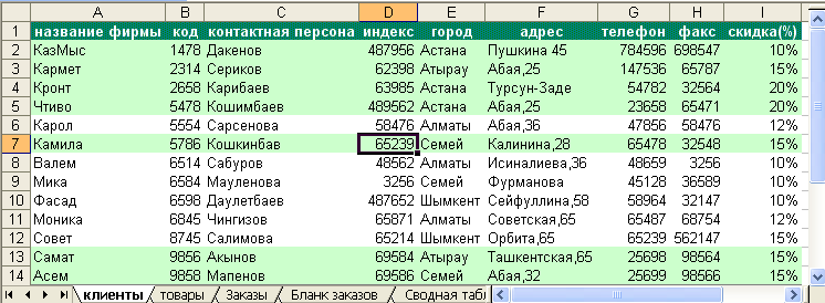
Sorting data. Must be selected from the menu Data  Sorting. Select the first sorting criterion in the dialog box Code and the second criterion City And OK.

Data filtering. Select from the menu Data  Filter/Atofilter. When you click on the name of this command, an arrow button will appear on the first row next to the heading of each column. It can be used to open a list containing all field values in a column. Select the name of one of the cities in City. In addition to field values, each list contains three more elements: (All), (First 10…) and (Condition…). Element (All) is designed to restore the display of all records on the screen after applying the filter. Element (First 10…) provides automatic display of the first ten entries in the list. If you are engaged in compiling all kinds of ratings, the main task which is to determine the top ten, use this function. The last element is used to form a more complex selection criterion in which conditional operators can be applied. AND And OR.

Place the cursor in any filled cell and do the following: in the menu Format  Auto Format  List 2 .

Creating a product list

The second list will contain data about the products we offer.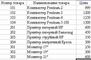

Lab #2

Sheet Orders

Rename the worksheet ListZ addressed Orders.

Enter the following data in the first line, which will be the field names in the future:
A1  Month of order , IN 1  order date , WITH 1  Order number , D1  Item Number , E1  Name of product , F1  Quantity , G1  price per one ., H1  Customer company code ., I1  Customer company name , J1  Order price , K1  Discount(%) , L1  Total paid .

For the first line do data alignment in the center Format cells alignment transpose by words .

Select columns one by one B, C, D, E, F, G, H, I, J, K, L and enter into field name names Date, Order, Number2, Item2, Quantity, Price2, Code2, Company2, Amount, Discount2 And Payment .

Highlight a column IN and execute the menu command Format cells. In the tab Number select
Numeric format date, and in the field Type select the format as HH.MM.YY. At the end of the dialogue
click the button OK.

Highlight columnsG, J, L and execute the menu command Format cells. In the tab Number
select Numeric format Monetary , indicate Number of decimal places equal to 0, and in the field
Designation select $ English (USA). At the end of the dialog, click the button OK.

Select column K and execute the menu command Format cells. In the tab Number select
Numeric formatPercentage , indicate Number of decimal places equal to 0. At the end
dialog click button OK.

In a cell A2 you need to type the following formula:

=IF(ISBLANK($B2)," ";SELECT(MONTH($B2),"January","February","March","April";"May"; "June"; "July"; "August"; "September"; "October"; "November"; "December")) (3.1)

And fill the cell in yellow.

Formula (3.1) works as follows; first, the condition for the emptiness of cell A2 is checked. If the cell is empty, then a space is put, otherwise, using the SELECT function, select the desired month from the list, the number of which is determined by the MONTH function.

To get the formula (3.1) do the following:

make the cell active A2 and call the function IF;

in the IF function window in the field Boolean_expression type manually $ B2="", V

field value_if_true type " " , in field value_if_false call the SELECT function;

in the function window CHOICE in field value1 type " January", in field value2 print

in field index_number and call the function MONTH;

in the MONTH function window in the field date_as_number dial the address $ B2 ;

Click the button OK.

To cell E2 we type the following formula:

=IF($ D2=" "; “ ”;LOOKUP($D2;Product number; Product name) (3.2)

Formula set rule:
Click in cell E2. Place the cursor on the icon of the Standard panel. A window will open Function master..., select the IF function. Follow the steps you see in the picture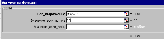

Those. in position Logic_expression click on a cell D2 and press the F4 key three times - get $D2, type =" ", use the Tab key or the mouse to move to the position value_if_true and dial. " ", move to the position value_if_false– click on the button next to the name of the function and select the command More functions.. → Categories → References and arrays, in the Functions window → VIEW→ OK → OK.

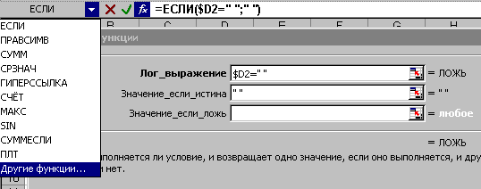
Function window will open VIEW. In position Lookup_value click on a cell D2 and press the F4 key three times - get $D2, use the Tab key or the mouse to move to the position Viewed_vector and click on the sheet label " Goods”, select a range of cells A2:A12, press the F4 key, go to position result_vector– click again on the sheet label “ Goods”, select a range of cells Q2:W12, press the F4 key, and OK. If you did everything right, it will appear in the cell # HD.

WITH

fill cell yellow color.

10. Into the cell G2 we type the following formula:

=IF($D2=" ";" ";LOOKUP($D2;Product number; Price)) (3.3)

Make a cell fill yellow color.

11. Into the cell I2 we type the following formula:
=IF($H2=" ";" ";LOOKUP($H2;Code; Firm)) (3.4)
Make a cell fill yellow color.

12. Into the cell J2 we type the following formula:
=IF(F2=" ";" ";F2* G2) (3.5)
Make a cell fill yellow color..

13. Into the cell K2 we type the following formula:
=IF($H2=" ";" ";LOOKUP($H2;Code; Discount)) (3.6)
Make a cell fill yellow color.

14. Into the cell L2 we type the following formula:
=IF(J2=" ";" ";J2- J2* K2) (3.7)
Make a cell fill yellow color.

15. Cells B2, D2 and H2 - in which there are no formulas, fill in blue color. Highlight a range A2 - L 2 and a fill handle ( black cross in the lower right corner of the block ) extrude fill and formulas up to 31 lines included.

16. Make the cell active AT 2 and drag down the fill handle to the cell VZ1 inclusive.

17. Into the cell C2 type in the number 2008-01, which will be the starting order number and drag down the fill marker to the cellCZ1 inclusive.

18. Now you need to fill in the columns from the keyboard Q2:W31 , D2: D31 And H2:H31. WITH AT 2 By AT 11 we collect January dates (for example, 01/2/08, 01/12/08). WITH AT 12 By AT 21 we collect February dates (for example, 12.02.08, 21.02.08) and from B22 By B31 we collect March dates (for example, 03/05/08, 03/06/08). IN D2: D31 we dial the numbers of goods i.e. 101, 102, 103, 104, 201, 202, 203, 204, 301, 302 and 303. The numbers can be repeated and go in any order, similarly in H2:H31 enter Codes your firms that you have typed on the sheet Clients. per column F enter two-digit numbers.

19.

(SRSP) Lab #3

Order form

In cell H5, enter the entry Code, and in a cell

=IF($

$3=" "; “ ”;VIEW($

$3;Order; Code2))

To cell C7 enter entry Name of product.

=IF($

$3=" "; “ ”;VIEW($

$3;Order; Product2)),

To cell H7 enter character № , and in a cell

=IF($

$3=" "; “ ”;VIEW($

$3;Order; Number 2))

To cell C9 enter entry Quantity ordered.

To cell E9-formula
=IF($ E

$3=" "; “ ”;VIEW($

$3;Order; Quantity))

units by price

Cell H9 must contain the formula
=IF($ E

$3=" "; “ ”;VIEW($

$3;Order; Price2)),

this cell should be given an underline and a currency style.

per unit

Type in C11 text Total Order Value, and in E11 put the formula
=IF($ E

$3=" "; “ ”;VIEW($

$3;Order; Sum)),

Discount(%)

11,

11, H11

Merge and center

=IF($

$3=" "; “ ”;VIEW($

$3;Order; Discount2)),

and set formatting options: underline and percentage style.

To cell C13-text To pay. And in a cell

=IF($

$3=" "; “ ”;VIEW($

$3;Order; Payment)),

and set formatting options: underline and currency style.

To cell E13 enter entry Designed by:, highlight E13,

13, H13,

Finally, set the column widths

Now in E3 indicate Order number, and before printing your form last name.

You have successfully completed the work, hand it over to the teacher!

pivot table

A list of orders for practical use has been created and its data is subject to analysis. The PivotTable Wizard will help us perform the analysis.

Pivot tables are created from a list or database.

8. You have successfully completed the work, hand it over to the teacher!

(SRSP) Lab. No. 4. Branches

Create a workbook and save it in your folder as Branches (your last name). Let's start the example by creating a table and entering data about each branch.

Preparatory stage. Copy to clipboard from sheet Goods books Orders data about goods, their numbers and prices, i.e. copy a range of cells A1-C12 sheet Goods.

Go to the first page of the book Branches and into the cell A3 paste the copied table fragment. In 3 order into cellsD3, E3, F3 enter the entries accordingly Number of orders, Quantity sold And Volume of sales. Set text centering in cells and allow word wrapping.

To cell F4 put the formula: \u003d C4 * E4 and copy it into cells F5- F14 .

Type in cell B15 word Total:, and in a cellF15 insert sum formula or click toolbar button Standard. excel it will determine the range of cells, the contents of which should be summarized.

There should be as many such sheets as you had cities in the sheet Clients. We have to copy this sheet 4 times.

To do this, place the mouse cursor on its label and press the right button of the manipulator. In the context menu, select the command Move/Copy, in the dialog box that appears, specify the sheet before which the copy should be inserted, activate the option Create a copy and press OK. It is much easier to copy with the mouse: position the mouse pointer on the sheet tab and move it to the copy paste position while holding down the key [ ctrl] .

Worksheet names match titles cities from the sheet Clients, For example, Almaty, Astana, Shymkent, Aktau, Karaganda or other names. Enter the name of the branch corresponding to the name of the sheet and into the cell A1 this sheet.

Complete the sheet Orders one more column. To cell M1 enter a word City. To cell M2 enter the formula =IF(ISBLANK($ H 2);“ ”;LOOKUP($ H2;Code; City)) , extend this formula to row 31 of that column.

Select from the menu Data  Filter/Atofilter. Select in column City first branch. Column DataQuantity sheet Orders will be entered by you in the columnQuantity sold book sheet Branches, in the lines corresponding to the item numbers. If goods with the same number are sold in different months, then their total quantity is taken. And so the sheets of all cities are filled.

Consolidation of data. Copy from the first page of the book Branches range A3-B14, go to worksheet 6 and paste in the cell A3.

Let's move on to consolidation. Set the cell pointer toC3 and select from the menu Data  Consolidation.

Listed Functions element must be selected Sum. Specify in the input field Link the range of cells whose data is to be consolidated. It is convenient to mark a range of cells with the mouse.

Place the input cursor in the field Link, click on the label of the first city, for example - Almaty, select a range of cellsD3- F14 and press the button Add window Consolidation. As a result, the specified range will be rearranged in the field List of ranges.

Then go to the sheet of the second city. The range is indicated automatically, press the button Add and so 5 times.

If the top row and (or) the left column contain headings that need to be copied to the final table, activate the corresponding options in the group Use labels. Since in our example the top row contains the column headings, we need to activate the option On the top line.

If a dynamic relationship is to be established between the source data and the data of the consolidated table, enable the option Create links to source data.

button Review should be used to select the file that contains the data to be consolidated.

Click the button OK.

To cell A1 enter the name of the new table Final data.

Type in cell B70 meaning Total:, and in E70 - and press the key [ Enter]

Now we proceed to determine the share of the total profit of the amount received from the sale of each product. Type in F9 formula = E9/$E$70 and copy it to the rest of the column F ( to the cell F70) .

Format column contentF in percentage style. The results obtained allow us to draw conclusions about the popularity of a particular product.

When consolidating data, the program writes each element in the final table and automatically creates a document structure, which allows you to ensure that only the necessary information is displayed on the screen and unnecessary details are hidden. Structure symbols are displayed to the left of the table. The numbers indicate the levels of the structure (in our example - 1 And 2). The plus sign button allows you to decrypt higher level data. Click for example button for cell A9 to get information about individual orders.

Copy formula fromF9 into cells F4- F8.

Numbers turn into Charts

Preparatory work. Since each chart needs its own table, let's create a new pivot table based on the sheet data Orders book of the same name Orders.

Open a previously created workbook Orders. Create a new workbook and give its first sheet a name Table . This sheet will contain the numerical material for the chart.

Place the pointer in the cell AT 3 and select menu Data  Pivot table.

Choose the first way to arrange data − In a list or database

Microsoft

excel

Further.

In the second step, placing the input cursor in the field Range followed by menu Window go to workbook Orders and worksheet Orders and highlight the range

Further

Structure should be defined pivot table. Place in area lines button Name of product, and in the region columns - button Month. Sum will be calculated by field Order price, those. move this button to the area data . Click the button Ready.

Highlight a range

Click the button Chart Wizard in the toolbar Standard.

In the first step, specify chart type, click on the button Further.

Confirm in the second step range =Table!$

$4:$

$15.

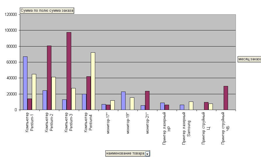
In the third step, specify chart options (Titles, Axes, Legends, etc.).Chart name enter Sales volume by month,Categories (X)- Name of product And Meaning(

)

Volume of sales(

USD

)

Sample,

Further.

Click on the button Ready.

Lab #1

The purpose of the work: to learn how to work with spreadsheets and learn how to build various diagrams.

Brief theoretical information

Excel is a spreadsheet program.

The interface of the Excel application window is similar to that of the Word application window (title bar, menu bar, toolbars, status bar). But a formula bar is added, which is not in Word.

There are two types of displaying an Excel document - “normal” and “page layout”, which can be set in the View menu.

Page settings are configured in the menu File/Page settings. Here you can also set the Header and Footer on the page. In the header, you can specify, for example, the group number, in the bottom - the student's full name. In the "Sheet" tab, you can configure the order in which pages are displayed.

Workbook. An Excel document is workbook , consisting of a set worksheets stored on disk in single file . By default, the workbook has 3 sheets. This number can be changed (up to 255) in the Tools/Options/General tab. Also, you can add or remove sheets to the book at any time (via the context menu with the right button). Sheets in the book can be glued (Kn. Shift + clicks on those sheets that need to be glued). The information written on the glued sheets is the same. For example, if you need to create the same table template on several sheets, you need to glue them together, create a table once, then “ungroup” the sheets through the context menu. All sheets that have been glued together will have the same table.

In addition to worksheets, a workbook can store charts based on data from one or more tables, and macros. A macro is a VisualBasic program that processes table data.

Links can be established between workbook documents, and changes made in one table are automatically fixed in all related documents. Excel also handles data prepared by various Windows applications.

Worksheet. Comprises electronic cells having an address: A1, B10, etc. The address of the current cell is displayed in the name field (leftmost field of the formula bar). The worksheets contain 256 columns and 65536 rows. Column headings –A…Z,AA…AZ,BA…BZ. Row headers: 1 to 65536.

Cell data. Two cells can be entered kind data: constant values and formulas . Constant values are entered directly into the cell, they do not change when copied. Formulas are used to organize calculations. When copying formulas data values change in the cells.

There are two representation cell data: in-machine and screen . In-machine is used for calculations, these are the internal values of the cells, and not displayed on the screen. The display representation is determined by the format of the cell.

Cells can contain the following data types :numbers, text, date and time, booleans, error values.

Numbers. The numbers are stored in the machine with the highest precision. The screen representation of a number is determined by the format: Format/ Cells/ Number/ Numeric formats. You can enter whole numbers, decimals, or numbers in exponential (exponential) form. If the cell is filled with characters (sharp), it means that the entered number exceeds the width of the column.

Text . This is any set of characters entered that Excel does not interpret as a number, date and time, Boolean value, or error value. You can enter up to 255 characters of text per cell. To enter a number as text in a formula, you must enclose it in quotation marks. ="45.00".

Text Formatting: Format/Cells/Tab Alignment, Font, Border, Appearance.

date and time .The date is represented in the machine as a number, determined by the number of days from the system date (1900) to the date represented in

cell. This can be seen if you select the "General" format in the cell with the date. The date 01/22/2005 is equivalent to the number of 38374 days from 01/01/1900, and the date 01/07/2005 is equivalent to the number 38359 days from 01/01/1900. Therefore, addition and subtraction operations can be performed on dates (in cells with the date "01/15/1900" and the number "15" there is a formula =A1-B1, which calculates the number of days between the dates "01/22/2005-01/07/2005". The difference is 15 ). Time is represented in the machine as a fraction. You can also see this if you select the "General" format in the cell over time. The time 16:14 is equivalent to the fraction 0.6763889.

The display representation of the date and time is also defined in the menu Format/Cells/Number/Number Formats. To quickly enter the current time in a cell, press Ctrl +<:>, and for the current date –Ctrl+<;>.

Boolean values take the values "true" and "false". These values are the result of logical and comparison operations.

Erroneous values are the result of erroneous calculations. Erroneous values begin with a sharp sign: n/a! (invalid value), link! (invalid reference), value! (wrong type of argument in the function), name! (does not understand the name), number! (cannot correctly interpret the formula in the cell), etc.

Cell range is a group of consecutive cells. Range references use the following address operations:

: (colon) - allows you to refer to all cells between the boundaries of the range, including

significant (A1:B15);

, (comma) - operator to combine ranges of cells or individual cells

ب (space) is an intersection operator that refers to common range cells,

Β5:B15ٮ A7:D7. In this example, cell B7 is shared between two ranges.

Entering, editing and formatting data.

Distinguish between direct data entry and the use of automation tools for entry.

Direct – direct data entry into the current cell. To complete the entry in the current cell and to move to the next cell, press one of the following keys

When you enter the same data into a range it is necessary: Select the range - Enter data in the active cell of the range - press Ctrl + Enter.

Input automation.

Editing.

Editing operations can be divided into the following two groups:

Editing introduced into a cell data . The contents of cells can be edited both directly in the cell (double-click on the cell) and in the formula bar (click on the right side of the formula bar), while the word "Edit" appears in the status bar. In this mode, all editing tools become available.

Editing at the level of cells, ranges, rows, columns. Basically, these are the editing commands of the "Edit" and "Insert" menus.

Formatting.

All commands for formatting data, rows, columns, sheets, etc. are concentrated in the "Format" menu.

Charts inexcel.

The diagram includes many objects, each of which can be selected and modified (edited and formatted) separately. When moving the mouse pointer over the chart, a tooltip appears next to it, indicating the type of object the pointer is near.

Chart Objects .Axis(X is the category axis, Y is the value axis). data point– one data item, for example, salary for January. Data series- a set of data points (clearly visible on the graph - all points of the data series are connected by one line). Legend– icons, patterns, colors used to distinguish data series. data marker– represents a data point on the chart as a rectangle, sector, point, etc., the type of marker depends on the type of chart; all markers of the same data series have the same shape and color. Text– all labels (chart title, values and categories on the axes) and labels (test associated with data points); for captions, you can use the "caption" icon on the drawing panel, or create floating text : click on one of the data rows - enter the test (it will appear in the formula bar) - press "Enter".

Rules , used by Excel default when building diagrams.

1. Excel assumes that the data series to chart is along the long side of the selected range of cells.

2. If a square range of cells is selected or it occupies more cells in width than in height, then the category names will be located in the top line of the range. If there are more cells in height than in width, then category names go down the left column. And if the cells that Excel will use as category names contain numbers (not text or dates), then Excel assumes that these cells contain a series of data, and numbers the category names as 1, 2, 3, 4, etc.

3. Excel assumes that the titles along the short side of the selection should be used as legend labels for each data series. If there is only one data series, then Excel uses this name as the title of the chart. And if the cells that Excel intends to use as legend labels contain numbers (not text or dates), then Excel assumes that these cells contain the first points of the data series, and assigns a name to each data series: “Series1”, “Series2”, etc. d.

Macros. Serves to automate repetitive operations in Excel. A macro consists of a sequence of internal Excel commands (macro). In Excel, a macro is created using the Tools/Macro/Start Recording command. This command allows you to create a macro using a macro recorder (a way to record a program). In parallel with user actions, the macro recorder logs user actions, automatically translating them into its own macro language. In this way, you can create relatively simple programs that run without user intervention.

Example: using a macro recorder to create a macro that builds a diagram of the dynamics of wages Ivanova A.P. by months. For this you need:

Assignments for laboratory work No. 1.

Create a spreadsheet on the instructions of the teacher.

Build two diagrams based on this table:

a histogram with one y-axis;
chart with the main and with the minor Y axes, while presenting two data series in the form of graphs.

Create a mixed chart in which one data series is presented as a histogram and the second data series is presented as a graph. Set the data series in the Word editor, save the file with the .txt extension, then import this file from the Excel program. The data is provided by the instructor.

Create a macro (on the instructions of the teacher).

Copyright JSC "Central Design Bureau "BIBCOM" & LLC "Agency Book-Service" Federal Agency for Education State Educational Institution of Higher Professional Education "Kazan State Technological University" Laboratory work on informatics MS EXCEL Guidelines Kazan 2006 Copyright JSC "Central Design Bureau "BIBCOM" & LLC "Kniga-Service Agency" UDC 658.26:66.094 Compiled by: Assoc. E.S. Vorobyov, Assoc. E.V. Nikolaeva, Assoc. F.I. Vorobieva Laboratory work in informatics. MS Excel: Method. instructions / Kazan. state technol. un-t; Comp.: E.S. Vorobyov, E.V. Nikolaev, F.I. Vorobyov. - Kazan, 2006. - 58 p. The basic methods of working in the MS Excel package are outlined, the procedure and rules for creating and editing spreadsheets and charts, performing basic calculations, sorting and filtering data, analyzing and summarizing data, and using logical expressions, summary and distribution functions, and matrix operations. A separate laboratory work is devoted to finding a solution to a one- and two-parameter problem. They can be used in the study of the disciplines "Informatics", "Use of computers in technology" and "Use of computers in calculations", can serve as a manual for extracurricular work of students, and can also be used by specialists of any subject area for independent development of computer technologies. Designed for full-time and correspondence forms training of specialties 240802.65 "Basic processes of chemical production and chemical cybernetics" and 240801 "Machines and apparatus of chemical production", students in the direction 2480800 "Energy and resource-saving processes in chemical technology, petrochemistry and biotechnology". Il. 68, tab. 1, bibliography. 5 names Prepared at the Department of General Chemical Technology. Published by decision of the editorial and publishing council of the Kazan State Technological University. Reviewers: B.K. Kurbatov, Associate Professor of KSTU. ON THE. Tupoleva E.A. Mukhutdinov, Associate Professor, Kazan State Technological University, Kazan State Technological University, 2006 Excel tables 1. Run Microsoft program Excel: click on the Start button; in the menu that appears, select Programs; select Microsoft Excel from the pop-up menu. 2. Carefully examine the Microsoft Excel window (Fig. 1). Many horizontal menu items and toolbar buttons are the same as menu items and buttons in the Word editor window. However, the workspace has a completely different look, which is a marked-up table consisting of cells of the same size. One of the cells is clearly selected (framed with a black frame - a table cursor). How to select another cell? To do this, just click on it with the mouse, and the mouse pointer in this Fig. 1 time should look like a light cross. Try highlighting different table cells. Use the scroll bars to move around the table. 3. In order to enter text into one of the cells of the table, you need to select it and immediately (without waiting, as in the Word processor for the text cursor) “write”. Select one of the cells in the table and “write” in it the name of today's day of the week. 4. The main difference between the work of spreadsheets and a word processor is that after entering data into a cell, they must be fixed, i.e. make it clear to the program that you have finished entering information -3- Copyright OJSC "Central Design Bureau" BIBCOM " & LLC "Agency Book-Service" in this particular cell. You can fix the data in one of the following ways: press the key (Enter); click on another cell; use the cursor keys on the keyboard (arrows). Record the data you entered. 5. Select the table cell containing the day of the week and use the paragraph alignment buttons. How is alignment done? Make a conclusion. After all the experiments, be sure to return the original alignment - to the left, in the future it will be important. 6. You have already noticed that the table consists of columns and rows, and each of the columns has its own heading (A, B, C ...), and all rows are numbered (1, 2, 3 ...) (Fig. 1). To select the entire column, just click on its header; to select the entire row, click on its header. Select the entire column of the table in which the name of the day of the week you entered is located. What is the title of this column? Select the entire row of the table in which the name of the day of the week is located. What is the title of this line? Use the scroll bars to determine how many rows the table has and what is the name of the last column. 7. Select the cell of the table that is in column C and line 4. Pay attention to the fact that in the "Name field" (Fig. 1), located above the heading of column A, the address of the selected cell C4 has appeared. Highlight another cell and you will see that the Address has changed in the Name field. What is the address of the cell containing the day of the week? 8. Let's imagine that in the cell containing the day of the week, you also need to add part of the day. Select the cell containing the day of the week, enter the name of the current part of the day from the keyboard, for example "morning", and fix the data by pressing the (Enter) key. What happened? Part of the day was not "added" to the cell, and the new data replaced the original data, and instead of the day of the week, you received part of the day. That is, if you select a table cell containing some data and enter new data from the keyboard, the table cell will contain the latest information. How to supplement the contents of a table cell (edit) without retyping all the data? If you select the cell containing the part of the day, you will see that its contents are duplicated in the "Formula Bar" located above the column headings (Fig. 1). It is in the "Formula Bar" that you can set the traditional text cursor with a mouse click, make all the required changes and then fix the final version of the data. Select the table cell containing the part of the day, place the text cursor in front of the text in the "Formula Bar" and re-type the day of the week. Fix the data. You should get the following picture (Fig. 2). -4- Copyright JSC "Central Design Bureau" BIBCOM " & LLC "Agency Book-Service" 9. It can be seen that the record went beyond its cell and occupied the Tuesday morning part of the neighboring one. This only happens when the adjacent cell is empty. Let's take it Fig. 2 fill in and check what changes. Select the cell of the table located to the right of the cell containing your data (the cell they "came to"), and enter any text into it. Now only that part of your data that fits in the cell is visible (Fig. Tuesday, Friday 3). How to view the entire post? And Fig. 3 again, the "Formula Bar" will come to your aid. It is in it that you can see all the contents of the selected cell. So, the "Formula bar" allows you to: make changes to the contents of the selected cell; view the contents of the cell if the record is not visible in its entirety. Select the cell containing the day of the week and part of the day, and view the full contents of the cell in the Formula Bar. 10. How can I increase the width of the column so that both the day of the week and part of the day are visible in the cell at the same time? To do this, move the mouse pointer to the right border of the column heading, "catch" the moment when the mouse pointer becomes a black double arrow, and holding down the left mouse button, move the column border to the right. The column has expanded. Similarly, you can change the line height. In this case, the cursor, when approaching the bottom edge of the row header, takes the form. Change the width of the column containing the day of the week and part of the day so that all the entered text is visible in the table cell. 11. It often happens that you need to select more than one cell and not a whole column, but a block of cells (several cells located side by side). 12. To do this, place the mouse pointer in the extreme cell of the selection and, with the left key pressed, move the mouse to the opposite edge of the selection (the entire selected block is "covered" by the frame, all cells, except for the one from which the selection began, are painted black) . Please note that during the selection process, the "Field of Name" registers the number of rows and columns that fall into the selection. At the same moment when you release the left key, the address of the cell from which the selection began is displayed in the "Name field". Select a block of cells, starting with cell A1 and ending with the cell containing "Friday". To select the entire table, use the "empty" corner button above the first row heading. -5- Copyright JSC "TsKB "BIBCOM" & LLC "Agency Book-Service" Select the entire table. Remove the selection by clicking on any cell. 13. How to delete the contents of a cell? To do this, just select a cell (or a block of cells) and press the (Delete) key or use the command of the horizontal menu "Edit" ⇒ "Clear". Delete all your entries. Exercise 2 Applying basic spreadsheet techniques: Entering data into a cell. Font formatting. Changing the column width. Autocomplete, formula entry, table framing, text alignment to the center of the selection, a set of subscripts and superscripts Let's make a table that calculates the nth term and the sum of an arithmetic progression. First, let us recall the formula for the nth member of an arithmetic progression: an = a1 + d (n − 1) and the formula for the sum of the first n members of an arithmetic progression: n S n = (a1 + an) ⋅ , 2 where a1 is the first member of the progression, and d is the difference of the arithmetic progression. On fig. 4 is a table for calculating the nth term and the sum of an arithmetic progression whose first term is -2 and the difference is 0.725. Rice. 4 Before doing the exercise, come up with your own arithmetic progression, i.e. e. Specify your own first term of the progression and difference. The exercise can be decomposed into the following steps: select cell A1 and enter the heading of the table “Calculation of the n-th term and the sum of an arithmetic progression” into it. The title will be placed in one line and will take several cells to the right of A1; in cell A2 enter "d", in cell B3 - "n", in C3 - "an", in D3 - "Sn". To set subscripts, first type all the text that should be in the cell (for example, an), then enter the "Formula Bar", select the text that should be a subscript (for example, n), open the command "Format" ⇒ "Cells ...” (there is only one “Font” tab in the dialog box that opens) and activate the “subscript” switch in the “Modify” group; Calculation of the nth term and the sum of the arithmetic progression d n an Sn 0.725 1 -2 -2 0.725 2 -1.275 -3.275 0.725 3 -0.55 -3.825 0.725 4 0.175 -3.65 0.725 5 0.9 -2.75 0.725 6 1.625 -1.625 7 2.35 1.225 0.725 8 3.075 4.3 0.725 9 3.8 8.1 0.725 10 4.525 12.625 -6- Copyright JSC "Central Design Bureau "BIBCOM" & LLC "Agency Book-Service" select the completed four cells. Use the appropriate toolbar buttons to increase the font size by 1 pt, center it, and apply bold character style. The table header is set. Now you can start filling in the table. 1. In cell A3, enter the value of the difference of the arithmetic progression (in our example, this is 0.725). 2. Next, you need to fill in a row of lower cells with the same number. It is uninteresting and irrational to type the same number in each cell. In the Word editor, we used the copy-paste technique. Excel makes it even easier to fill cells with the same data. Select cell A3, which contains the difference of the arithmetic progression. The selected cell is bordered by a frame, in the lower right corner of which there is a small black square - a fill handle. If you bring the mouse pointer to the fill marker, and at the moment when the mouse pointer takes the form of a black cross, drag the fill marker down several cells (in this case, a hint appears to the right of the cursor, what value is entered in the current cell), then the entire row of selected cells will be filled with the data located in the first cell. Fill in, thus, nine more cells below cell A3 with the value of the difference of the arithmetic progression. 3. The next column contains a sequence of numbers from 1 to 10. And again, the fill marker will help us fill in the row. Enter the number 1 in cell B3, the number 2 in cell B4, select both of these cells and, grabbing the fill handle, drag it down. The difference from filling with the same data is that by selecting two cells, you indicated the principle by which the remaining cells should be filled. The fill marker can be dragged not only down, but also up, left or right, and the fill will spread in the same directions. The fill element can be not only a formula or a number, but also text. You can enter "January" in the cell and, filling in the row further to the right, get "February", "March", and "stretching" the fill marker from the "January" cell to the left, respectively, get "December", "November", etc. Try doing this outside of the table you're creating. Most importantly, before spreading the selection, select exactly the cell (or those cells) on which the filling is formatted. 4. The third column contains nth members progressions. Enter in cell C3 the value of the first term of the arithmetic progression. In cell C4, you need to put a formula for calculating the nth member of the progression, which consists in the fact that each cell of the column differs from the previous one by adding the difference of the arithmetic progression. All formulas start with an equal sign. To enter a formula into a cell, you must: activate the cell; -7- Copyright OJSC "TsKB" BIBCOM " & LLC "Agency Book-Service" enter the "=" sign from the keyboard or click on the "Change formula" button in the formula bar; enter (without spaces) the required values or references, as well as the necessary operators; fix input. The cell address is entered into formulas in Latin case. If the entry was made in the Russian case, then the error message "#NAME?" appears. Select cell C4 and type in it the formula = C3 + A4 (do not forget to switch to Latin, and instead of referring to cell A4, you can enter the specific value of the difference of your arithmetic progression). You can not type from the keyboard the address of the cell to which the link is made. After typing the equal sign, click on cell C4 and its address will appear in the formula bar, then continue typing the formula. In this case, you do not need to switch to Latin. Having fully entered the formula, fix it by pressing (Enter), the result of the calculation will be in the cell, and the formula itself in the "Formula Bar". Another function of the “Formula Bar” appeared: if in a cell you see the result of calculations using a formula, then the formula itself can be viewed in the “Formula Bar” by highlighting the corresponding cell. If you typed a formula incorrectly, you can correct it in the Formula Bar by first selecting the cell. Select cell C4 and, similarly to filling the cells with the difference of the progression, fill in the formula by dragging the fill handle down, a row of cells, below C4. Select cell C8 and look in the Formula Bar to see what the formula looks like, it looks like =C7+A8. It is noticeable that the references in the formula have changed relative to the offset of the formula itself. 5. Similarly, enter the formula = (-2 + C3) * B3 / 2 in cell D3 to calculate the sum of the first n members of an arithmetic progression, where instead of -2 there should be the first member of your invented arithmetic progression. Select cell D3 and fill the lower cells with formulas by dragging the fill handle down. 6. Now all the cells are filled with data, it remains only to arrange them. All columns are the same width, although they contain information of different sizes. You can manually (using the mouse) change the width of individual columns, or you can automatically adjust the width. To do this, select all table cells containing data (not entire columns, but only a block of filled cells without the heading "Calculate the nth term and the sum of an arithmetic progression") and execute the command "Format" ⇒ "Column" ⇒ "AutoFit Width". 7. Now let's format the heading of the table "Calculation of the n-th term and the sum of an arithmetic progression". Select cell A1 and apply bold characters to the contents of the cell. The heading rather unaesthetically "crawls out" to the right beyond the limits of our small plate. -8- Copyright OJSC "Central Design Bureau "BIBCOM" & LLC "Agency Book-Service" Select four cells from A1 to D1 and execute the command "Format" ⇒ "Cells ...", select the tab "Alignment" and set the switches (Fig. 6): group "Alignment" ⇒ "horizontally:" to the position "center of selection"; group "Display" ⇒ "Wrap by words". This will allow you to arrange the title in several lines and in the center of the selected block of cells. The table was almost brought to the 8. kind of sample. If at this moment you execute the view "File" ⇒ "Preview", then it turns out that it remains to frame the table. To do this, select the table (without a title) and execute the command "Format" ⇒ "Cells ...". In the dialog box that opens, select the "Border" tab, define the line type and activate the "Top", "Bottom", "Left", "Right" switches (Fig. 5). This procedure applies to each of the cells in the selected area. Then select the block of cells related to the header: from A1 to D2 and, having done the same operations, set the "External" switch. In this case, a border is obtained around all selected cells, and not each. Perform a review. Rice. 5 Fig. 6 -9- Copyright OJSC "Central Design Bureau "BIBCOM" & LLC "Agency Book-Service" Laboratory work №2 Exercise 1 Consolidation of basic skills in working with spreadsheets, familiarity with the concepts: data sorting, types of text alignment in a cell, number format Consignor and his address The consignee and his address To the Register No. Date of receipt "___" ___________200__. INVOICE No. 123 dated 11/15/2000 Supplier Trading House "Roga and Hooves" Address 243100, Klintsy, st. Pushkina, 23 R / account No. 45638078 in MMM-bank, MFO 985435 Additions: No. Name Unit of measurement 1 2 3 4 5 6 TOTAL Head of the enterprise Quantity Price Amount Sidorkin A.Yu. Chief Accountant Ivanova A.N. The exercise consists in creating and filling out a commodity invoice form. It is best to divide the exercise into three stages: Stage 1 - creating a table of the invoice form; 2nd stage - filling in the table; 3rd stage - registration of the form. 1st stage Consists in creation of the table. The main task is to fit the table to the width of the sheet. To do this: pre-set the margins, size and orientation of the paper ("File" ⇒ "Page Setup ..."); - 10 - Copyright OJSC "Central Design Bureau "BIBCOM" & LLC "Agency Book-Service" by executing the command "Service" ⇒ on the "Parameters ..." tab, in the group of switches Parameters of the window, activate the switch "Auto pagination" (Fig. 7) As a result, you will get the right border of the dialing bar in the form of a vertical dotted line (if it is not visible, move with the horizontal scroll bar Fig. 7 to the right) and the bottom border of the dialing bar in the form of a horizontal dashed line (in order to see it move with vertical stripe scroll down). Auto pagination allows you to keep track of which columns fit on the page and which do not, already in the process of data entry and table formatting. № 1 2 3 4 5 6 Name Unit of measurement Quantity Price Amount TOTAL Pic. 8 Create a table according to the proposed sample with the same number of rows and columns (Fig. 8). Align and format the font in the header cells, adjust the width of the columns by changing it with the mouse. Enter the numbering in the first column of the table using the fill handle. "Line" the table using lines of various thicknesses. Note that in the last row, five adjacent cells do not have an inner frame. The easiest way to achieve this is the following way: select the entire table and set the frame - "External" with a thick line; - 11 - Copyright JSC "Central Design Bureau "BIBCOM" & LLC "Agency Book-Service" then select all lines except the last one and set the frame with a thin line "Right", "Left", "Top", "Bottom"; after that, select separately the rightmost cell of the bottom row and set the “Left” frame for it with a thin line; it remains to select the first row of the table and set the “Bottom” frame for it with a bold line. Although you can do the opposite. First, "line" the entire table, and then remove the extra framing lines. At this stage, it is advisable to execute the command "File" ⇒ "Preview" to make sure that the table fits entirely on the sheet in width and all the border lines are in the right place. 2nd stage It consists in filling in the table, sorting the data and using various number formats. Fill in the columns "Name", "Quantity" and "Price" as you wish. Set the currency format of the number in the cells where the amounts will be placed and set the required number of decimal places, if any. In our case, these are the cells of the columns "Price" and Fig. 9 "Amount". You need to select them and execute the command "Format" ⇒ "Cells ...", select the "Number" tab and select the "Currency" category (Fig. 9). This will give you a division into thousands to make it easier to navigate large amounts. Enter the formula for calculating the amount, which is to multiply the price by the quantity, and fill in the row of cells down with the formula. Enter the formula in the cell for the grand total. To do this, select a block of those cells that you want to add, and one empty cell under this block, in which you want to place the result. After that click on the toolbar button. Try changing the data in individual cells and see how the result of the calculation changes. Sort the entries alphabetically. To do this, select all the rows of the table, except for the first (header) and last ("Total"), you can not select and numbering. Execute the “Data” ⇒ “Sort...” command (Fig. 10), select the column by which you want to sort the data (in our case, this is column B, since it contains the list of goods to be sorted), and set the switch to Ascending position. 3rd stage of the invoice, insert For additional lines before the table. To do this, select the first few rows of the table and execute the command "Insert" ⇒ "Rows". Rice. 10 The same number of rows as you selected will be inserted. Type the required text before and after the table. Watch out for alignment. Please note that the text "Date received '__'_______200_" and the names of the heads of the enterprise are entered in the same column in which the column of the table "Amount" is located (the rightmost column of our plate), only right alignment is applied. The text "ACCOUNT No. ..." is entered in the cell of the leftmost column, and alignment is applied to the center of the selection (the cells of one row are pre-selected across the entire width of the account table). A border has been applied to these cells at the top and bottom. All other textual information before and after the table is entered in the leftmost column, left alignment. Perform a review. Exercise 2 Introducing the concept of "absolute reference", setting the exact value of the column width using the horizontal menu commands. Inserting a Function Using the Function Wizard The new concept of "absolute reference" can be seen with a concrete example. Let's prepare a traditional table of squares of two-digit numbers (Fig. 11), so familiar to everyone from the algebra course. In cell A3, enter the number 1, in cell A4 - the number 2, select both cells and drag the selection handle down to fill the column with numbers from 1 to 9. Similarly, fill cells B2 - K2 with numbers from 0 to 9. When you filled in the line with numbers from 0 to 9, then all the cells you need to work are not visible on the screen at the same time. Let's narrow them down, but so that all columns have the same width (which cannot be achieved by changing the width of the columns with the mouse). To do this, select columns from A to K and execute the command "Format" ⇒ - 13 - Copyright OJSC "Central Design Bureau "BIBCOM" & LLC "Agency Book-Service" "Column" ⇒ "Width ...", in the input field "Column width » Enter a value, for example 5. Of course, everyone understands that in cell B3 you need to put a formula that squares the number made up of the tens indicated in column A and the units corresponding to the value placed in row 2. Thus, the number itself, which should be squared in cell B3, can be specified by the formula A3 * 10 + B2 (the number of tens multiplied by ten plus the number of ones). It remains to square this number. 1 2 3 4 5 6 7 8 9 0 100 400 900 1600 2500 3600 4900 6400 8100 1 121 441 961 1681 2601 3721 5041 6561 8281 tables 2025 2704 2809 2916 3025 3844 3969 4096 4225 5184 5329 5476 5625 6724 6889 7056 7225 8464 8649 8836 9025 6 256 676 1296 2116 3136 4356 5776 7396 9216 7 289 729 1369 2209 3249 4489 5929 7569 9409 8 324 784 1444 2304 3364 4624 6084 7744 9604 9 361 841 1521 2401 3481 4761 6241 7921 9801 11 Let's try to use the "Function Wizard". To do this, select the cell in which the calculation result (RT) should be placed, and execute the command "Insert" ⇒ "Function ..." (Fig. 12). The "Function Wizard (Step 1 of 2)" dialog box (Figure 12) has two subwindows: "Category" and "Function". When you select a specific function, a brief description of the function appears at the bottom of the dialog box. Among the proposed Fig. 12 categories of functions, select "Math", among "Functions" - "Degree", press the Ok button. In the next dialog box (Fig. 13), enter in the "Number" field (base of the degree) - A3 * 10 + B2 and in the "Exponent" field - 2. As well as when typing the formula directly in the cell of the spreadsheet, no the need to enter from the keyboard the address of each cell referenced by the formula. In the dialog box of the second step of the "Function Wizard", it is enough to point the mouse at the corresponding cell of the spreadsheet, and its address will appear in the "Number" input field of the dialog box. You will have to enter only arithmetic Fig. 13 signs (*, +) and the number 10. In cases where you need to select cells closed by a window to enter arguments, there are buttons to the right of each field for entering arguments that allow you to collapse and expand the dialog box. In addition, the "Function Wizard" window can be moved to the side by "grabbing" the title bar with the mouse. In the same dialog box (Fig. 13) you can see the value of the number itself (10) and the result of calculating the degree (100). It remains only to press the Ok button. In cell B3, the result of the calculation appeared. I would like to extend this formula to the rest of the table cells. Select cell B3 and fill in the adjacent cells by dragging the fill handle to the right. What happened (Fig. 14)? Rice. 14 Why didn't the result meet our expectations? In cell C3, the number is not visible, because it does not fit entirely in the cell Expand column C with the mouse. The number appeared on the screen, but it clearly does not correspond to the square of the number 11 (Fig. 15). Rice. 15 Why? The fact is that when we extended the formula to the right, Excel automatically changed the cell addresses, taking into account our offset, to which the formula refers, and in cell C3, not the number 11 is squared, but the number calculated by the formula B3 * 10 + C2. In all previous exercises, we were quite satisfied with relative references to table cells (when the formula is moved according to the same law, the references also shift), but here it became necessary to fix certain references, i.e. indicate that the number of tens can be taken only from column A, and the number of units only from line 2 (in order to make the formula possible - 15 - Copyright JSC "Central Design Bureau "BIBCOM" & LLC "Agency Book-Service" spread down). To do this, Excel has the ability to set absolute and mixed references. An absolute reference is a reference that does not change when formulas are copied. To do this, a dollar sign $ is added before the column name and row number (either entered from the keyboard, or after entering the cell address, the F4 function key is pressed). Mixed links are links that are only partially absolute, i.e. either a column or a row is fixed. In this case, the dollar sign $ is placed either before the letter, in the case when a column is fixed, or before the digit, in the case when a row is fixed. The dollar sign $ is either entered from the keyboard, or after entering the cell address, the F4 function key is pressed until the $ sign is in the required place. When you copy a formula containing a mixed reference, only the relative part of the reference changes. Return the width of column C to its original position and do the following: Select cell B3 and, setting the text cursor in the "Formula Bar", correct the existing formula =POWER(A3*10+B2;2) to the correct one =POWER($A3*10+ At $2.2). Now, using the services of the fill marker, you can fill in all the free cells of the table with this formula (first drag the fill marker to the right, then, without removing the selection from the resulting block of cells, down). We used mixed references to enter cell references for column A and row 2 data. The absolute reference in our example could be used if we entered into the formula not the number 10, by which the numbers in column A are multiplied, but the address of the cell, for example A15 (where we would enter this number 10). In this case, the formula in cell B3 would be written as: =POWER($A3*$A$15+B$2) and then copied to the rest of the cells as well. Try this. It remains to arrange the table: enter the heading in cell A1, format it and center it on the selection, frame the table and fill individual cells with the background. Exercise 3 Introducing the concept of "cell name" Imagine that you have your own company that sells some products and you have to print out a price list every day with prices for goods depending on the dollar exchange rate. Prepare a table consisting of columns: "Product name"; "Equivalent to $US"; "Price in rubles". - 16 - Copyright JSC "Central Design Bureau "BIBCOM" & LLC "Agency Book-Service" Fill in all columns, cream "Price in rubles". Fill in the "Product name" column with text data (the list of goods at your discretion), and fill in the "US$ equivalent" column with numbers (prices in $). It is clear that in the column "Price in r." the formula should be placed: “Equivalent to $ US” * “Dollar exchange rate”. Why is it inconvenient in this formula to multiply by a specific exchange rate value? Yes, because with each change in the course, you will have to change your formula in each cell. It is easier to take it under the value of the dollar separate cell , which is referred to in the formula. It is clear that the reference must be absolute, i.e. the value of the dollar exchange rate can only be taken from this particular cell with a fixed address. We discussed how to set absolute references above, however, there is another convenient way: to refer not to the cell address, but to the name that can be assigned to the cell. When naming a cell or range of cells, you can access that cell or range at any time and from anywhere in the table, even if they change their location or are on different sheets. Select the cell in which the dollar rate will be entered (above the table), enter the value of the dollar rate for today in it and execute the command "Insert" ⇒ "Name" ⇒ "Assign ...". In the dialog box that opens (Fig. 16), you can enter any name and select the range for which this name is entered in the "Formula" field. The name can be up to 255 characters long and contain letters, numbers, underscores (_), backslashes (\), periods, and question marks. However, the first character must be a letter, an underscore (_), or a backslash (\). Names that are perceived as numbers or cell references are not allowed. In the dialog box that appears, you just have to enter the name of the cell (its exact address is already given in the "Formula" input field) and click the OK button. Please note that in the "Field of the name", instead of the address of the cell, its name is now placed. In the cell located to the left of the "Dollar_rate" cell, you can enter the text "Dollar rate". Rice. 16 Now it remains to enter the formula for calculating the price in rubles. To do this, select the topmost empty cell of the "Price in rubles" column and enter the formula as follows: enter the "=" sign, then click on the cell located to the left (which contains the price in dollars), then enter the sign "*" and "Exchange_dollar". The formula should look something like this: =B7*USD_rate. Fill the formula down using the fill handle. Select the appropriate cells and apply the currency number format to them. Style the table header: center align, apply bold font style, expand the row and apply vertical center alignment using the command "Format" ⇒ "Cells ...", select the tab "Alignment" and in the group "Vertical:" select " In the center." In the same dialog box, activate the "Wrap by words" switch in case some heading does not fit on one line. Change the column widths. Select the table and set a frame for it. - 18 - Copyright OJSC "Central Design Bureau "BIBCOM" & LLC "Agency Book-Service" Laboratory work No. 3 Exercise 1 Changing the orientation of the text in the cell, familiarization with the capabilities of the databases excel data. Sorting data by multiple keys Imagine that you are the owner of a small store. It is necessary to keep a strict record of the receipt and consumption of goods, to have a real balance in front of your eyes every day, to be able to print the name of the goods by department, etc. Even in such a difficult task, Excel can make the job much easier. Let's smash this exercise for several tasks in a logical sequence: creating a table; filling the table with data in the traditional way and using a form; selection of data according to a certain attribute. 1. Creating a table Enter the table headings in accordance with the suggested pattern. Please note that the heading is located in two lines of the table: in the top line “Income”, “Expense”, “Balance”, and the rest of the heading items in the line below (Fig. 17). Remaining amount Remaining Remaining amount Quantity of expense Expense Price of expense Product name Quantity of receipt Department Price of receipt No. Unit of measure Incoming 1 2 3 4 5 6 Pic. 17 Entering title text is best to start on the second line. You have already noticed that the "Incoming" column covers two cells. The word “Income” is typed in the same column as “Income Price”, then two adjacent cells are selected, and the text is centered on the selection (this operation was repeatedly considered in previous exercises). The cells "Expense" and "Remainder" are formatted similarly. Select the second title row and center align. You can also see that in order for the entire table to fit in the width of the sheet, in some cells the text is “rotated 90°”. Select those cells in which you want to "expand" the text and select the "Format" ⇒ "Cells ..." command on the "Alignment" tab (Fig. 18) select "Text Orientation" 90o and be sure to activate the switch "Wrap by words" (leave the vertical alignment "Bottom"). For the remaining (non-expanded) cells, apply the vertical alignment "Centered". Set the border of the table ("Format" ⇒ "Cells ...", tab "Border"). Install in cells, Fig. 18 containing prices, monetary number format (“Format” ⇒ “Cells…”, “Number” tab). Enter the numbering of the table rows (column No.), using the fill marker. Insert formulas for the amount of the balance ("Incoming Quantity" minus "Expense Quantity") and the balance amount ("Remaining Quantity" times "Output Price"). Extend these formulas down the table. In the process of performing a task, in many cases it is more convenient to use the context menu called by pressing the right mouse button. So, to format cells, it is enough to select them, right-click at the moment when the mouse pointer is inside the selection and select the command "Format" ⇒ "Cells ...". This will take you to the same Format Cells dialog box (Figure 18). Yes, and editing the contents of the cell (correcting, changing data) is not at all necessary in the "Formula Bar". If you double-click on a cell or press the F2 key, a text cursor will appear in it and you can make any necessary corrections. 2. Filling in the table Rename "Sheet1" to "Availability". To do this, right-click on the label "Sheet1" and select the command to rename. Enter a new name and press the (Enter) key. Decide what type of product you are going to sell, and what departments will be in your store. Enter data in the table not by department, but mixed (in order of receipt of goods). Fill in all cells except those containing formulas ("Remainder"). Be sure to leave the last line of the table blank (but this line must contain all formulas and numbering). Enter the data in such a way that there are different goods from the same department (but not in a row) and there must be goods with zero balance (all sold) (Fig. 19 ). Agree that the traditional way of filling out the table is not particularly convenient. Let's take advantage of Excel databases. 1 2 3 4 5 6 Department Confectionery Dairy Meat Meat Wine and vodka Product name Marshmallow in chocolate Cheese Sausage Moscow Balyk Vodka "Absolute" Consumption Remaining Incoming price Incoming quantity Expenditure quantity Expenditure quantity Remaining amount Remaining amount № Unit of measurement Arrival pack. 20 p. 15 kg. 65 p. 10 kg. 110 r. 20 kg. 120 r. 10 bottles 2 l. 400 r. 100 25r. 85 p. 120r. 140 r. 450 r. 15 8 15 5 99 0 2 5 5 1 0 0 170 r. 600 r. 700 r. 450 r. 0 r. Rice. 19 Select the command "Data" ⇒ "Form..." You will get a data form (Fig. 20) containing static text (names of database fields) and edit windows in which you can enter and edit text. Calculated fields (in which formulas are placed) are displayed without editing windows (“Remaining Quantity” and “Remaining Amount”). Now you have your table as if in the form of separate record cards (each of which represents a table row). Rice. 20 You can move between records either by using the buttons "Previous", "Next", or by the cursor keys (up, down), or by moving the slider on the scroll bar of the data form. Reaching up to last entry (we left it empty on purpose, but extended formulas and numbering to it), fill it with new data. It is convenient to move between the editing windows in which data is entered using the (Tab) key. When you have completed the entire entry, press the (Enter) key and you will automatically be taken to a new blank entry card. As soon as you fill in a new record, all the information you entered will automatically be reproduced in the original table. Fill in a few new entries and click the Close button. - 21 - Copyright JSC "Central Design Bureau "BIBCOM" & LLC "Agency Book-Service" As you can see, it is quite convenient to fill in the table in the form mode. 3. Filling in the table using a ready-made list of data Since we have a limited number of departments and their names are constant, it is best to use a pre-prepared list of these departments when filling out the table. Erase the names of departments from the column "Department" and enter a short list that includes the names of all departments once, outside the table, for example, in column L. Then select the cells of the column "Department" in the table and select the command "Data" ⇒ "Check". This will bring up Fig. 21 dialog box "Validation of input values" (Fig. 21), where we must specify the conditions for verification. In our example, we must choose from the list (which we enter in the "Data Type" field). To select the “Source” of data, use the window minimization button. Press it, highlight the list of our departments in column L and return to the window using the maximize window button. After completing these steps, click the Ok button. Now, when moving to the cells of the “Department” column, where the verification condition is set, a square with an arrow will appear to the right of these cells, by clicking on which we can select the name of the department we need (Fig. 22). Rice. 22 To hide the departments table, you can make the font in the cells of column L white, or hide the entire column. To hide column L, select it, choose Format ⇒ Column ⇒ Hide. To return column L to the screen, select the columns around the hidden column (columns K and M) and execute the command "Format" ⇒ "Column" ⇒ "Display ". Note that the "Hide" command can also be applied to strings. To do this, a line is selected, the command "Format" ⇒ "Line" ⇒ "Hide" is selected. To return a line to the screen, you need to select the lines around the hidden line and execute the command "Format" ⇒ "Line" ⇒ "Display". Rice. 23 You can also create a list on another sheet. However, in this case, it is impossible to specify addresses that include the sheet name as the "Source" of information, i.e. you must enter the name of the range of cells as the address. In the last lesson, we got acquainted with how to set the name of a single cell. To set a name for cell ranges, you must select the range of cells, not just one cell, before executing the command "Insert" ⇒ "Name" ⇒ "Assign". Let's transfer our list of departments from column L of Sheet1 to Sheet2 to column A. Select the cells in which our list is placed and execute the command "Insert" ⇒ "Name" ⇒ "Assign". In the dialog box that opens (Fig. 23), you can enter any name, for example, "Department", and select the range for which this name is entered in the "Formula" field (by default, the address of the range we selected is placed here). After that, press the Ok button. Now in the dialog box of the "Check ..." command as a source (Fig. 21) it is enough to enter the sign "=", then press the F3 key to open the list of available cell names, select "Department" in the list that opens and press the Ok buttons to close the dialog boxes . 4. Sorting data So, you filled in the table in the order of receipt of goods, but you would like to have a list of goods by departments, for this we apply row sorting. Select the table with the second row of the header, but without the first column "No.", and select the command "Data" ⇒ "Sort..." (Fig. 24). Rice. 24 - 23 - Copyright OJSC "TsKB "BIBCOM" & LLC "Agency Kniga-Service" Select the first sorting key: in the "Sort by" drop-down list, select "Department" and set the switch to the "Ascending" position (all departments in the table will be located alphabetically). If you want all products within the department to be placed alphabetically, then select the second sorting key: in the "Then by" drop-down list, select "Product name", set the switch to "Ascending". Now you have full list goods by department. 5. Filtering data Let's continue our acquaintance with the possibilities of Excel databases. Recall that on a daily basis we need to print a list of goods left in the store (having a non-zero balance) or show the balance in some department, but for this we first need to get such a list, i.e. filter the data. Highlight the table with the second header row (as before creating the data form). Select the menu command "Data" ⇒ "Filter..." ⇒ "AutoFilter". Deselect the table. Each table header cell now has an arrow button (it is not printed) that allows you to set the filter criterion (Fig. 25). Rice. 25 Suppose we want to leave all entries for the "Confectionery Department". Expand the list of cells "Department" and select "Pastry". In this case, Excel will change the table and display it in a view where only the data related to the selected department will be present (Fig. 26), and the arrow in the column where the autofilter was applied will turn blue. Rice. 26 - 24 - Copyright OJSC "Central Design Bureau "BIBCOM" & LLC "Agency Book-Service" In the same way, you can view data for other departments or select a filtering criterion in another column. The table can be printed in filtered form. Filtered lines can be highlighted with font color, background, frames, or otherwise formatted. By removing the filtering, we get a very visual layout of the table. In the filtered section of the table, you can calculate sums, products, and perform other operations as if there were no other rows in the table. For example, we want to calculate the amount of the balance in the confectionery department. To do this, we select the data of the "Remainder Amount" column, capturing the last free cell, and press the "Auto Sum" button. The function SUBTOTALS(9; F2:F8) will appear in a free cell (Fig. 26). In it, the first argument is the number of a mathematical or statistical operation (1 calculation of the average; 2 and 3 - counting the number of numbers and non-empty cells; 4 and 5 - calculating the maximum and minimum; 6 - product; 7 and 8 - standard deviation; 9 - sum ; 10 and 11 are the variance), and the second is the calculation interval. The SUBTOTAL function is located in the category of mathematical and differs in that it calculates values only for visible cells, and does not take into account invisible ones. When you change the filtering, the subtotals also change (Fig. 25), while the usual summation or product function will remain unchanged. Let's change the condition of the problem a bit, let's say we want to see data on non-zero residues of the confectionery department. To do this, select the "Condition" item in the list of the "Balance Amount" column. This will bring up the Custom AutoFilter dialog box (Fig. 28). In the upper field, select "more" "0.00r.". The result obtained is shown in fig. 28. Fig. 27 Now, let's say we want to look at data on non-zero balances in the confectionery and meat departments. To do this, we leave the same filter in the “Balance Amount” column, and select “Condition” in the “Department” column (Fig. 28). In the upper field, select "equal to" Fig. 28 - 25 - Copyright JSC "TsKB "BIBCOM" & LLC "Agency Kniga-Service" "Confectionery", below "equals" "Meat", and set OR as a logical function. The result obtained is shown in fig. 29. Fig. 29 To see the whole table again, you need to click on the arrow in the column where the filtering was applied (they are shown by blue arrows), select "All" in the list, or once again go to the "Filter" ⇒ "Auto Filter" command of the "Data" menu to cancel the mode filtration. - 26 - Copyright OJSC "Central Design Bureau "BIBCOM" & LLC "Agency Book-Service" Laboratory work No. 4 Exercise 1 Creating and editing graphs in Excel document Very often in life you have to measure the dependence of one variable on another and show these dependences in the form of graphs. Excel provides the possibility of such a visual display of numerical electronic data. Suppose some experiment was carried out, for example, the dependence of some parameter on temperature was measured. The initial temperature was 10°C. The step of change is 10оС. Enter this information on excel sheet (Fig. 30). To place the title "Initial data" above the table of initial data as shown in Fig. 30 is shown in the figure, select two cells, execute the command "Format" ⇒ "Cell Format ..." and on the "Alignment" tab, check the box "wrap by words", "merge cells" in the display and alignment group "centered" and horizontally, and vertically (see Lab #1). Now let's prepare a table of experimental data (Fig. 31). Enter the data of the first column - numbers in order are entered using the fill marker (black dot in the corner of the table cursor). The heading of the "Temperature" column is entered according to the formula: =A2 (i.e. in the formula there is a link to the cell address, Fig. 31 where the name of the parameter is placed in the table "Initial data" (Fig. 30)). The initial temperature is equal to the initial temperature, i.e. =B2. Further, it differs from the previous one by a step. Therefore, in the second line, the temperature is equal to the initial temperature + step, i.e. =E3+$B$3. To further use the fill handle to copy the formula, and the step must be taken constantly from the same cell, we make the reference to it absolute. The information introduced in this way allows us to automate the adjustment of the table of experimental data to changes in the initial conditions. Try instead of "temperature" in the initial data, enter "pressure", and set the initial value, for example, 20. The values of Yekper should be taken from the experiment, so just enter them from the keyboard. To format the title "Experiment" it is best to use the format copying option. To do this: - 27 - Copyright OJSC "Central Design Bureau" BIBCOM " & LLC "Agency Book-Service" Pic. 32 Fig. 33 select the cell "Initial data"; Click on the Format Standard Paint Bar tool button. In this case, Excel copies the format of the selected cell, and the mouse pointer turns into a brush, to the left of which there is a plus sign; drag the mouse pointer over the range of cells where you want to copy the selected format. To plot Yexper versus temperature, select these two columns, including their headers, and choose Insert ⇒ Chart or click the Chart Wizard button on the toolbar. The first dialog box "Chart Wizard (Step 1 of 4) - Chart Type" (Fig. 32) has two tabs - "Standard" and "Custom". At this stage, a variant of the diagram under construction is selected from the available samples. To build a graph of the dependence of one quantity on another, you need to select the "Point" chart type, and then any of its five types. Let's just draw dots and not draw lines. Click on the "View result" button (Fig. 32). Excel will immediately show how our data will be displayed on the finished chart. To go to each subsequent step of the Chart Wizard, use the "Next" button. In the second window "Chart Wizard (Step 2 of 4): Chart Data Source" on the "Data Range" tab, the address of the selected range of source data and a sample of the chart being built are displayed (Fig. 33). Select "in columns" and click the "Next" button. - 28 - Copyright JSC "Central Design Bureau "BIBCOM" & LLC "Agency Book-Service" At the third stage of the Chart Wizard (at step 3) in the "Chart Parameters" window (Fig. 34) determine the nature of the diagram design - perform its formatting. The third window of the Chart Wizard has the following tabs: title - allows you to enter the text of the chart title and axis labels; axes - allows you to define Fig. 34 display and marking of coordinate axes; grid lines - allows you to define the type of lines and the nature of the grid display; legend - allows you to show or hide the legend and determine its place on the chart. Legend - Fig. 35 is a small sub-window on the diagram, which displays the names of data series and examples of their coloring on the diagram (in the form of a Legend key); data labels – allows you to control the display of labels corresponding to individual data elements on the chart; data table - allows you to add or hide the data table used to build the chart on the chart. The last (fourth) window of the diagram wizard (Fig. 35) is used to determine its placement in the workbook. It is recommended to choose its placement on a separate sheet, because. in this case, the diagram is easier to insert into other documents, it does not block the original data, it is more readable, etc. Once you have defined all the required parameters, click the "Finish" button. Excel built a chart for us (Fig. 36) using a certain set of parameters, such as the color of the construction area (the area in which the chart itself is displayed, without titles, legends and other elements), font, scales, point size, etc., default. To change one or another chart formatting option, you need to right-click on it and select the appropriate command in the context menu that opens. Make the background of the plotting area white. To do this, right-click on the plotting area of the diagram and select the "Format plotting area" command. In the dialog box that opens (Fig. 37), check the switch in the "normal" fill group. Click the Ok button. - 29 - Copyright JSC "Central Design Bureau "BIBCOM" & LLC "Agency Book-Service" Y=f(x) 12 10 8 Y 6 4 2 0 0 20 40 60 80 100 120 X Yexper Fig. 36 Fig. 37 Fig. 38 Increase the size of the dots. To do this, right-click on the points and select the "Format Data Series" command. In the dialog box that opens (Fig. 38), in the “size” group, set the size of the dots, for example, 8 pt. Here you can also select other data parameters, for example, change the marker, i.e. type of points, draw a line by selecting its color, thickness and type, smooth the line, etc. Our function argument changes from 10 to 100, and the scale on the X axis has a minimum value of 0 and a maximum of 120. In addition, the font of the data label is small . How to change it? Right-click the X axis and select Format Axis. In the dialog box that opens (Fig. 39), on the “Scale” tab, set the minimum value - 10, the maximum - 100 and the price of the main divisions - 10, because our data changes in steps of 10. In the same window, on the Font tab, you can increase the font size and change its style, for example, increase it to 8 pt and make italic. On the "Alignment" fold, you can set the vertical writing of signatures. Similarly, you can - 30 - Copyright JSC "Central Design Bureau "BIBCOM" & LLC "Agency Book-Service" format the Y-axis. Do it. Have you already understood the principle of chart formatting? Then increase the font size of the title, adjust the legend, titles of the axes. An example of a formatted chart is shown in the figure (Fig. 40). To predict the values of the response - parameter Y at the output of the experiment from the factor - independent variables X at the entrance to the system (in our case, this is temperature), it is necessary to know the functional dependence Y = f (X). Excel has the ability to automatically select such a function. Rice. 39 Yexper Y=f(x) 12 10 8 Y 6 4 2 100 90 80 70 60 50 40 30 20 10 0 X 40 Right-click on the points and select Add Trendline from the context menu. In the dialog box that opens (Fig. 41), on the Type tab, select the trend line type. Usually, a second-order polynomial trend line is used to describe the system: Y = a0 + a1 * X + a2 * X 2 , (1) where ai are the coefficients of the equation. If necessary, you can change the degree to 6. Then the equation will take the form: - 31 - Copyright JSC "Central Design Bureau "BIBCOM" & LLC "Agency Book-Service" Y = a0 + a1 * X + a2 * X 2 + a3 * X 3 + + a4 * X 4 + a5 * X 5 + a6 * X 6 . (2) Fig. 41 Fig. 42 On the "Parameters" tab, set the radio buttons to "show the equation on the diagram" and "put the approximation confidence value on the diagram" (Fig. 42). This will allow you to see the equation and the accuracy of the approximation of our data. The equation and accuracy displayed on the screen can be moved to any place in the diagram (as well as other inscriptions, for example, the title of the diagram, the names of the axes, the legend), by “grabbing” the frame with the left mouse button. An approximate final form of our dependence is shown in Fig. 43. Save the results of exercise 1, we will need them later (see Lab #6 below). y = -0.0054x2 + 0.6014x - 5.9667 R2 = 0.9817 Y=f(x) Yexp Polynomial (Yexp) 12 10 8 6 Y 4 2 0 -2 10 20 30 40 50 60 X 43 - 32 - 70 80 90 100 Copyright JSC "TsKB "BIBCOM" & LLC "Agency Kniga-Service" Exercise 2 Creating and editing surfaces in an Excel document In the previous exercise, we considered the possibility of visualizing a one-parameter dependence (the function depends on only one variable). In reality, such simple dependencies are quite rare. More often you have to deal with multi-parameter functions. How to visualize them, consider the example of a two-parameter problem. Let us have an equation: Z = sin X 2 − Y 2 + 5 ⋅ X ⋅ Y , (3) where X and Y change from -5 to 5 in increments of 1. It is necessary to plot the surface of the obtained Z values. To do this, you first need build a data matrix (Fig. 44). () Rice. 44 In cell B1, enter the first value Y = -5. Then execute the command "Edit" ⇒ "Fill" ⇒ "Progression ...". In the dialog box that opens (Fig. 45), set: "Location" - by lines, "Step:" equal to 1 and "Limit value:" equal to 5. After that, click the Ok button. In exactly the same way Fig. 45, the X values in column A are filled in, with the only exception that "Location" must be in columns. Execute it. After the argument values are entered into the table, fill in cell B2 with the formula to calculate Z (3). The Sin function is in the math category "Function Wizards". - 33 - Copyright OJSC "TsKB "BIBCOM" & LLC "Agency Kniga-Service" Do not forget that the formula must contain mixed references, since the X values must always be selected from column A, and the Y values from row 1. To fill in the entire tables, use the fill handle. The data for plotting the surface is ready, it remains only to plot them on the diagram. As in the previous exercise, we will use the "Chart Wizard" (Fig. 32 - 35). First, select the matrix of function values (you don't need to select the X and Y values in Fig. 46!), open the chart wizard in any way you know, and select the "Surface" chart type. Further, the construction of the surface from the construction of the graph is no different. The final diagram will look like the one shown in Fig. 46. You can rotate or adjust the diagram in the Format 3D Surface dialog box (Fig. 47), which is shown in Fig. 47. 47 is opened by right-clicking on the walls of the surface and selecting the context menu item "3D view...". - 34 - Copyright OJSC "Central Design Bureau "BIBCOM" & LLC "Agency Book-Service" Laboratory work №5 Exercise 1 Boolean expressions in Excel Let's enter the formula =7>5 into cell A1. It will return TRUE. Let's copy the contents of A1 to A2 and fix the formula in A2: =3>5. This formula will return FALSE. The right parts of both formulas are statements, i.e. statements about which one can infer whether they are true or not. Let's consider another example. Enter the number 2 in cell A4, and the formula =A4>3 in cell B4. The formula returns FALSE. Enter the number 6 in A4. The formula returns TRUE. B4 contains a predicate, i.e. statement with variables (in this case, there is only one variable). Depending on the value of the variables, the predicate can take the values TRUE and FALSE. In this example, the formula, as it were, answers the question: “Is the number (or the result of calculations using a formula) stored in cell A4 greater than 3?” Depending on the value of A4, the answer will be YES (TRUE) or NO (FALSE). In the formula =A4>3, its constituent parts (A4 and 3) can be considered arithmetic expressions, only very simple ones. A more complex example: =(A4^2-1)>(2*A4+1). You can omit the parentheses in this expression because arithmetic operations have higher precedence than comparison operators, but the parentheses make the formula more readable. The comparison operations are summarized in Table. 1. Table 1 > greater than >= greater than or equal< <= меньше или равно меньше = <>equals not equal Note that the greater than or equal to relation symbol is represented by two signs: > and =. The reason is that there is no ≥ sign on the keyboard. The statement and the predicate have a common name - a logical expression. Available logical operations, which allow you to build complex logical expressions. These operations are implemented in Excel as functions (NOT, AND, OR). At logic functions arguments can only take two values: TRUE and FALSE. A NOT function can have only one argument, while AND and OR functions can have two or more arguments. Example 1 In cell A1 (named z), write any number. Find out if it belongs to the segment . Solution. Give cell A1 the name z (Insert ⇒ Name ⇒ Assign). Let us introduce the number 3 into A1. In order for z to belong to the segment , it is necessary that two predicates be simultaneously true: z ≥ 2 and z ≤ 5 . In cell B1 we place the formula =I(z>=2;z<=5). Для ввода в формулу имени ячейки нажмите F3 для открытия списка имен. В В1 получим значение ИСТИНА. Следует предостеречь от неверного решения: формулы =2<=z<=5. Введите эту формулу в С1 и убедитесь, что она возвращает ЛОЖЬ! Коварство этой, на первый взгляд, такой естественной формулы в том, что Excel ничего не сообщает о ее некорректности. Пример 2 В ячейке А1 (с именем z) записано число. Выяснить, принадлежит ли оно одному из лучей на числовой оси: (-∞,2) или (5,∞). Решение. Для того чтобы z принадлежал хотя бы одному из лучей, нужно, чтобы был истинным хотя бы один из предикатов: z < 2 или z >5. In cell D1, place the formula =OR(z<2;z>5). A1 contains the number 3, so the formula returns FALSE. The problem could have been solved differently, taking into account the fact that the worksheet contains a formula for checking whether the number z belongs to the segment . The two rays mentioned make up the addition to this segment on the numerical axis. Let's enter the formula = NOT (B1) into cell E1. Verify by entering different numbers in cell A1 that the formulas in cells D1 and E1 produce identical results. In practice, "in its pure form" logical expressions, as a rule, are not used. The logical expression serves as the first argument of the IF function: IF(log_expression, value_if_true, value_if_false) The second argument contains the expression that will be evaluated if the logical_expression returns TRUE, and the third argument contains the expression that is evaluated if the logical_expression returns FALSE. Example 3 1. Enter in cell A2 a formula that returns z+1 if z >1 and z otherwise: = IF(z>1;z+1;z). (In the Function Wizard, IF is in the "Boolean" category, as well as the AND, OR, NOT functions.); 2. If z > 60, then in cell B2 display the message “Threshold value exceeded”, otherwise display z: =IF(z>60;"Threshold value exceeded";z) Please note that the text in the formulas is entered in quotation marks . 3. If z ∈ , then return z if z< 10, то возвращать 10, если z >25, then return 25. The expression for this condition will look something like this (we write the formula in C2): =IF(z<10;10;ЕСЛИ(z<=25;z;25)) Теперь попробуйте менять значение z в ячейке А1, следя за тем как меняются значения в ячейках с формулами. - 36 - Copyright ОАО «ЦКБ «БИБКОМ» & ООО «Aгентство Kнига-Cервис» Упражнение 2 Итоговые функции в Excel Некоторые функции Excel возвращают одно значение, в то время как аргументом имеют блок или несколько блоков. Такие функции будем называть итоговыми. Наиболее часто используемой из таких функций является СУММ − для ее ввода на панели «Стандартная» даже размещена специальная кнопка. Эта функция как бы подводит итог колонке чисел − отсюда и название для всей группы. Эти функции входят в категории «Статистические» и «Математические». Функция СУММ допускает до 30 аргументов. Поэтому с ее помощью можно находить сумму чисел из нескольких блоков. Допустима, например, такая формула =СУММ(В2:В9;12;-4.96;А4:С18). Если в блоке в какой-либо ячейке находится текстовое значение, то оно считается равным нулю. Кроме суммы к итоговым функциям относятся, например: МАКС и МИН − вычисление максимального и минимального значений, СРЗНАЧ − среднее арифметическое значение и т.д. Прочие итоговые функции вы можете найти в «Справке». К итоговым можно отнести функции И и ИЛИ. Пример 4 данные Имеются метеостанции – количество осадков (в мм) (Рис. 48). Необходимо получить суммарное, максимальное, минимальное и среднемесячное количество осадков. Решение. Введите формулы: в В17 =СУММ(В3:В14); в В18: =МАКС(В3:В14); в В19: =МИН(В3:В14); в В20: =СРЗНАЧ(В3:В14). Далее эти формулы скопированы в С17:D20. В блоке Е17:Е20 подведены итоги за три года. В Е17 формула =СУММ(В17:D17), в Е18: т.д. На =MAKC(B18:D18) и Рис. 48 Рис. 49 - 37 - Copyright ОАО «ЦКБ «БИБКОМ» & ООО «Aгентство Kнига-Cервис» результаты наложен формат: одна цифра после десятичного разделителя (кнопка «Уменьшить разрядность»). Существует две полезные функции, примыкающие к итоговым: СЧЕТЕСЛИ и СУММЕСЛИ. Их названия показывают, что они считают и суммируют не все данные, а только удовлетворяющие некоторому критерию. Функция СЧЕТЕСЛИ (интервал; критерий) подсчитывает в интервале (т.е. блоке) количество значений, удовлетворяющих критерию. Пример 5 Вычислим количество засушливых месяцев, т.е. месяцев, когда выпадало менее 10 мм осадков (Рис. 49). В ячейке В22 формула =СЧЕТЕСЛИ(В3:В14;"<10"). Критерий взят в двойные кавычки, как текстовая строка. Формула скопирована в C22:D22. В Е22 подсчитана сумма. Функция СУММЕСЛИ(интервал;критерий;сумм_интервал) устроена сложнее. Значения, удовлетворяющие критерию, выбираются из блока, заданного первым аргументом, суммируются соответствующие значения из сумм_интервал, заданного третьим аргументом. Если третий аргумент опущен, то суммируются ячейки в аргументе интервал. Предположим, нужно вычислить суммарные осадки, которые выпали в незасушливые месяцы. Дополним таблицу (Рис. 49). В ячейку В23 введена формула =СУММЕСЛИ(B3:B14;">=10"), then copied to C23:D23. This function can be used to solve a more difficult problem: what was the total amount of precipitation in 1993 in those months that were dry in 1994. The solution is given by the formula =SUMIF(D3 :D14;"<10"; С4:С15), которая возвращает значение 128,6. Поместите ее в ячейку В24. К итоговым можно отнести еще две функции: НАИБОЛЬШИЙ(блок;k) и НАИМЕНЬШИЙ(блок;k). Первая из этих функций возвращает k-e наибольшее значение из множества данных, а вторая − наименьшее. Пример 6 В ячейки A1:D1 введем набор чисел. В блок А2:А5 введем формулы, которые показаны в соседнем столбце Рис. 50 (Рис. 50). Для понимания работы функции важно отметить, что третье наибольшее значение в блоке не 2, как можно было бы подумать, а 6, т.е. совпадает со вторым наибольшим значением. И еще: если в блоке n элементов, то функция НАИБОЛЬШИЙ(блок,n) возвращает минимальное значение, что мы и видим в примере. Обратите внимание, что в А2:А5 получен исходный массив чисел, отсортированный по убыванию. Если в исходном блоке изменить какое-либо число, - 38 - Copyright ОАО «ЦКБ «БИБКОМ» & ООО «Aгентство Kнига-Cервис» то блок А2:А5 будет автоматически перестроен. В этом отличие от операции сортировки, которая проводится самим пользователем при необходимости. Обязательно сохраните результаты примеров 4-6, так как мы будем их использовать позднее. Упражнение 3 Табличные формулы в Excel Табличные формулы − очень мощное средство Excel, позволяющее в формулах обращаться с блоками, как с обычными ячейками, давать компактные решения сложных задач. В некоторых задачах вообще невозможно обойтись без табличных формул. Пример 7 Пусть нам известна сумма прихода и сумма расхода. Необходимо вычислить доход как разность этих величин. Введите исходные данные (Рис. 51). Рис. 51 В ячейку D2 можно набрать формулу: =В2-С2, а затем скопировать ее в D3:D5. В этих ячейках появятся формулы =В3-С3 и т.д. Однако здесь фактически из вектор-столбца В2:В5 вычитается вектор-столбец С2:С5. Поэтому можно непосредственно вычесть из вектора вектор одной формулой, а не создавать отдельные формулы для компонент вектора. Создание имен. Для наглядности дадим векторам имена. Выделите диапазон со вторым и третьим столбцами таблицы (В1:С5) и дайте команду меню «Вставка» ⇒ «Имя» ⇒ «Создать». Диапазон В2:В5 получит имя «Приход», а диапазон С2:С5 имя «Расход». Ввод табличной формулы с использованием имен диапазонов. Прежде мы вводили формулу в отдельную ячейку. А сейчас введем ее в диапазон. Подробно опишем шаги. Выделим блок D2:D5. В этом блоке активна ячейка D2. Наберем знак равенства =. Нажмем функциональную клавишу F3. Появится диалоговое окно «Вставка имени». Выберем имя «Приход» и щелкнем Оk. Формула примет вид: =Приход. Наберем знак минус -. Вновь нажмем клавишу F3. В диалоговом окне «Вставка имени» выберем имя «Расход» и щелкнем Ok. Формула примет вид: =Приход-Расход. Нажмем сочетание клавиш Shift+Ctrl+Enter. Во всех ячейках блока появится формула {=Приход-Расход}. - 39 - Copyright ОАО «ЦКБ «БИБКОМ» & ООО «Aгентство Kнига-Cервис» Прокомментируем шаги. На третьем и пятом шаге мы выбирали имя из списка имен. Можно было ввести имя непосредственно с клавиатуры, но предложенный метод проще и нет риска ошибиться в наборе имени. На шестом шаге мы нажимаем не Enter, как ранее при вводе формулы, a Shift+Ctrl+Enter (при нажатии клавиши Enter должны быть нажаты обе клавиши Shift и Ctrl). Это очень важно. Если бы мы нажали Enter, то формула была бы введена только в активную ячейку блока D2 (Проверьте!). Фигурные скобки, окружающие формулу, говорят о том, что это табличная формула. Эти скобки нельзя набирать вручную (формула будет воспринята как текст). Ввод табличной формулы. Разумеется, табличную формулу можно вводить и без использования имен. Скопируйте блок А1:С5 в А8:С12. Повторите все шаги. Выделите блок D9:D12. В этом блоке активной ячейкой является D12. Наберите знак равенства =. Выделите блок В9:В12, наберите знак минус -, выделите блок С9:С12, нажмите сочетание клавиш Shift+Ctrl+Enter. Во всех ячейках блока появится формула {=В9:В12-С9:С12}. Мы получили две идентичные таблицы. Выделение блока с табличной формулой. Выделите одну из ячеек блока и нажмите клавишу F5 (эквивалент пункта меню «Правка» ⇒ «Перейти»). В диалоговом окне щелкните по кнопке «Выделить», установите переключатель «Текущий массив». Изменение табличной формулы. Попытайтесь очистить одну из ячеек, занятую табличной формулой. Например, выделите ячейку D8 и нажмите клавишу Del. В этом случае должно появится сообщение «Нельзя изменять часть массива». Удалить блок можно только целиком. Отредактировать формулу можно так: выделить блок с формулой, нажать функциональную клавишу F2, внести изменения в формулу, нажать сочетание клавиш Shift+Ctrl+Enter. (Попробуйте, например, ввести формулу {=Приход-Расход-1}, потом отмените это.) Коррекция табличной формулы при увеличении блока. Добавьте в обе таблицы на рабочем листе строку с данными: Год - 1996, приход - 240, расход – 200. Необходимо посчитать прибыль за 1996. Раньше, когда формулы записывались в отдельные ячейки, мы бы поступили просто: скопировали бы формулу из ячейки D5 в D6. Проделаем это для первой таблицы. Вместо ожидаемого 40 получим результат 50, т.е. число из первой ячейки блока с табличной формулой. Та же операция для второй таблицы даст правильный результат 40, но в строке формул мы увидим {=В13:В16-С13:С16} – образовался второй блок, что вовсе не входило в наши планы. Удалим формулы в ячейках D6 и D13. Правильное решение для первой и второй таблиц разное. Для первой таблицы изменим именованные блоки (выделим В1:С6 и «Вставка» ⇒ «Имя» ⇒ «Создать», для каждого имени Excel задаст вопрос: «Заменить» существующее определение имени?» Отвечаем «Да»). Выделяем D2:D6, нажимаем клавишу F2 (редактирование) и, ничего не изменяя в формуле, нажимаем клавиши Shift+ Ctrl+Enter. Для второй таблицы выделяем D8:D13, нажимаем клавишу F2 и редактируем формулу. Выделим в формуле подстроку В8:В12 и выделим блок В8:В13, также поступим с блоком С8:С12 либо просто заменим в адресах блоков цифру 2 на цифру 3. Нажимаем сочетание клавиш Shift+Ctrl+Enter. - 40 - Copyright ОАО «ЦКБ «БИБКОМ» & ООО «Aгентство Kнига-Cервис» Коррекция табличной формулы при уменьшении блока. Теперь мы хотим удалить в каждой из таблиц строку для 1996 г. Для первой таблицы вновь изменяем поименованные блоки (в ячейке D6 результат отображается как #Н/Д - недоступно). Выделяем блок с табличной формулой, нажимаем клавишу F2 и добавляем в самое начало формулы апостроф (он расположен на клавише с буквой "Э"). Формула превращается в текст. Вводим этот текст во все ячейки (клавиши Ctrl+Enter). Табличная формула прекратила существование. Очищаем последнюю строку таблицы. Выделяем блок D2:D5, нажимаем клавишу F2, удаляем апостроф, нажимаем клавиши Shift+Ctrl+Enter. Аналогично поступаем со второй таблицей. Как видим, процедура непростая и неприятная. Для решения задачи проще было воспользоваться простыми формулами. Но применение табличных формул, как мы убедимся, дает такие дополнительные возможности, что с неудобствами, связанными с изменениями этих формул, придется смириться. Упражнение 4 Дистрибутивные функции в Excel В Excel можно к блоку применить функцию (большое множество функций Excel), с тем, чтобы она вернула новый блок, содержащий значения функции для элементов исходного блока. Пример 8 Пусть в блоке А1:А4 записаны числа 1, 4, 9, 16. Поместим в B1:В4 табличную формулу {=КОРЕНЬ(А1:А4)}. Будет выведен столбец значений: 1, 2, 3, 4. Можно считать, что функция КОРЕНЬ была применена к вектору из четырех компонент и вернула новый вектор. (Разумеется, тот же результат можно было получить, записав в В1 формулу =КОРЕНЬ(А1) и скопировав ее в блок В2:В4.) Теперь рассмотрим функцию, которую нельзя применять к блоку. Поместим в D1:D2 логические значения ИСТИНА и ЛОЖЬ. В блок Е1:Е2 запишем табличную формулу {=И(D1:D2;”ИСТИНА”)}. Эта формула вернет значение ЛОЖЬ во всех ячейках блока Е1:Е2. Получается, что функцию КОРЕНЬ можно применять к массиву, а функцию И – нет. Функции, которые можно применять к списку, называются дистрибутивными. Продолжим пример с вычислением квадратного корня от элементов блока. Мы хотим вычислить сумму корней ∑ ai . Поместим в ячейку В5 формулу =СУММ(В1:В4). Результат, разумеется, 10. А теперь вычислим эту же сумму, не используя промежуточный блок В1:В4. Поместим в ячейку А5 табличную формулу {=СУММ(КОРЕНЬ(А1:А4))}. Обратите внимание, хотя формула возвращает значение в одной ячейке, она должна вводиться как табличная, т.е. ее ввод заканчивается нажатием комбинации клавиш Shift+Ctrl+Enter. Для сравнения введите в А6 эту формулу как обычную, – она вернет сообщение об ошибке #ЗНАЧ!. - 41 - Copyright ОАО «ЦКБ «БИБКОМ» & ООО «Aгентство Kнига-Cервис» Итак, к массиву, возвращаемому дистрибутивной функцией, можно применить итоговую функцию, которая возвращает всего одно значение. Но вводить такую формулу нужно как табличную. Пример 9 Рис. 52 Функцию ИЛИ можно использовать в табличных формулах, но как итоговую, т.е. если ИЛИ имеет всего один аргумент и этот аргумент – блок. Пусть в блоке А1:В2 находятся названия планет (Рис. 52). В ячейку D2 введем табличную формулу {=ИЛИ(СОВПАД(А1:В2;D1))}. Функция СОВПАД возвращает логическое значение ИСТИНА или ЛОЖЬ в зависимости от совпадения или несовпадения своих аргументов – текстовых строк. Если бы в А4:В5 была введена формула массива {=СОВПАД(А1:В2;D1)}, то она вернула бы четыре значения (Рис. 52). Функция ИЛИ(А4:В5) возвращает значение ИСТИНА. Эти две формулы мы объединяем в одну табличную формулу, которую и ввели в D2. Пример 10 Вернемся к задаче обработки данных метеостанции (пример 4 и пример 5). Для расчета количества засушливых месяцев, т.е. месяцев, когда выпало менее 10 мм осадков, очень удобно использовать функцию СЧЕТЕСЛИ. Однако с ее помощью нельзя получить количество месяцев, на протяжении которых количество осадков лежало бы в диапазоне от 20 до 80 (назовем такие месяцы нормальными). Для этого необходимо использовать дистрибутивные функции. Скопируйте текст из ячейки А22 в ячейку А25 и откорректируйте его: «Количество нормальных месяцев». Сначала подсчитаем месяцы с нормальным количеством осадков. Будем использовать вспомогательный блок F3:H14 тех же размеров, что и блок с исходными данными. В ячейку F3 вводим формулу =ЕСЛИ(И(В3>20;B3<80);1;0) и копируем ее в остальные ячейки блока F3:H14. В блоке выводятся нули и единицы. Введенная формула является индикаторной функцией множества нормальных месяцев, т.е. 1 – выводится, когда количество осадков лежит в пределах между 20 и 80 мм и 0 – в противном случае. Остается подсчитать сумму таких месяцев. Для этого введем в ячейку F25 формулу =СУММ(F3:F14) и скопируем ее в блок G25:H25. А теперь решим эту же задачу без использования вспомогательного блока. Введем в В25 табличную формулу {=СУММ(ЕСЛИ(В4:В15>20;IF(B4:B15<80;1;0);0))} и скопируем ее в C25:D25. (Таким образом, машина, перебирая значения в указанном блоке, проверяет больше или меньше текущее число 20 и, если оно меньше, прибавляет к исходному число 0. В противном случае – проверяет выполнение второго условия (менее 80). Если и второе условие выполняется, то к исходному числу прибавляет 1. В противном - 42 - Copyright ОАО «ЦКБ «БИБКОМ» & ООО «Aгентство Kнига-Cервис» случае – 0). Формула {=СУММ(ЕСЛИ(И(В4>20;B4<80);1;0))} не приведет к успеху, так как функция И не является дистрибутивной). Этот пример очень важен. Он Рис. 53 дает рецепт, как подсчитать в множестве количество элементов, удовлетворяющих определенному критерию. Нужно составить на основе вложенных функций ЕСЛИ индикаторную функцию подмножества и применить к ней итоговую функцию СУММ, введя формулу как табличную. Теперь вычислим суммарное количество осадков, выпавших в эти месяцы Введите в А26 текст «Осадки в нормальные месяцы», в В26 – табличную формулу {=СУММ(ЕСЛИ(В3:В14>20; IF(B3:B14<80;В3:В14;0);0))} и скопируйте ее в C26:D26. В E25 и Е26 введите формулы для суммирования значений в строках (выделите блок В25:Е26 и щелкните кнопку «Автосумма»). Вы получите блок, показанный на рис. 53. Пример 11 В блоке А1:А10 записана числовая последовательность. Проверьте, является ли она возрастающей. Решение. Перейдите на новый лист. Запишите любую последовательность чисел в блок А1:А10. Окончательное решение можно записать одной формулой (поместите его в ячейку A12). {=ЕСЛИ(СУММ(ЕСЛИ(А2:А10-А1:А9>0;1;0))=COUNT(A1:A10)1;"increasing";"is not increasing")) Now let's analyze this formula: A2:A10-A1:A9 A8 is subtracted from A9, etc.) - forms a block consisting of the first differences of the elements of the original block; IF(А2:А10-А1:А9>0;1;0) – makes up a block of indicators of positive first differences; SUM(IF(A2:A10-A1:A9>0;1;0)) – counts the number of non-zero elements in the block of indicators; COUNT(А1:А10)-1 – calculates the size of the block of indicators equal to the size of the original block reduced by 1; if the number of non-zero elements in the block of indicators is equal to the size of the block of indicators, then the sequence is increasing, otherwise it is not. Try to build the corresponding blocks and the final functions from them in stages in order to achieve a clear understanding of how the final formula is composed. - 43 - Copyright OJSC "Central Design Bureau "BIBCOM" & LLC "Agency Book-Service" Exercise 5 Matrix operations in Excel The simplest operations that can be performed with matrices: addition (subtraction), multiplication by a number, multiplication, transposition, calculation inverse matrix . Example 12 Matrix addition and matrix multiplication by a number. Add matrices M and N, where − 1 0 4  2 − 3 7 M = and N =   2 − 3 5 .    − 1 5 6 Solution. We introduce the matrices M and N into the blocks A1:C2 and E1:G2. In block A4:C5 we introduce a tabular formula (=A1:C2+E1:G2). Note that the selected block has the same dimensions as the original matrices. What happens if you select block A4:D6 before entering the formula? #N/A will appear in the "extra" cells, i.e. "Unavailable". And if you select A4: B5? Only part of the matrix will be displayed, without any messages. Check. Using names makes entering a spreadsheet formula much easier. Give the ranges A1:C2 and E1:G2 the names M and N, respectively (execute the command for each block "Insert" ⇒ "Name" ⇒ "Assign"). In block E4:G5, enter the tabular formula (=M+N). The result, of course, should be the same. Now let's calculate the linear combination of 2M-N matrices. In block A7:C8 we introduce a tabular formula (=2*M-N). You should get the following results:  5 − 6 10 1 − 3 11 M +N = and 2 M − N = − 4 13 7  .    1 2 11 The above examples lead us to the conclusion that the usual operation of multiplication in relation to blocks is not quite equivalent to multiplication of matrices. Indeed, for matrix operations in Excel there are functions included in the category "Mathematical": MOPRED - calculation of the determinant of the matrix; MOBR - calculation of the inverse matrix; MULTIP - matrix multiplication; TRANSPOSE - transposition. The first of these functions returns a number, so it is entered as a regular formula. The rest of the functions return a block of cells, so they must be entered as tabular formulas. The first letter "M" in the name of the three functions is an abbreviation for the word "Matrix". Example 13 Calculate the determinant and inverse matrix for the matrix - 44 - Copyright JSC "Central Design Bureau "BIBCOM" & LLC "Agency Kniga-Service" − 73 78 24 A =  92 66 25 .   − 80 37 10  Check the correctness of the calculation of the inverse matrix by multiplying it by the original one. Repeat these steps for the same matrix, but with element a33=10.01. Solution. Let's place the original matrix in block A1:C3. In cell B5 we put the formula for calculating the determinant = MOPRED (A1: C3). In block A7:C9 we introduce a formula for calculating the inverse matrix. To do this, select the block A7:C9 (it has three rows and three columns, like the original matrix). Let's introduce the formula (=MOBR(A1:C3)). Even if you are using the Function Wizard, you must complete your input by pressing the Shift+Ctrl+Enter key combination (instead of clicking the OK button). If you forgot to pre-select block A7:C9, and entered the formula in cell A7 as a regular Excel formula (finished by pressing Enter), then you do not need to enter it again: select A7:C9, press F2 (edit), but do not change the formula , just press the keys Fig. 54 Shift+Ctrl+Enter. Copy block A1:C9 to block E1:G9. Slightly change one element of the original matrix: in cell G3, instead of 10, enter 10.01. Changes in the determinant and in the inverse matrix are striking! This specially chosen example illustrates the numerical instability of the calculation of the determinant and inverse matrix: a small perturbation at the input gives a large perturbation at the output. For further calculations, we will assign the names to the matrices on the worksheet: A1: C3 - A, A7: C9 - Ainv, E1: G3 - AP, E7: G9 - APinv. In order for these names to appear in already entered formulas, select the corresponding formulas, select the menu item "Insert" ⇒ "Name" ⇒ "Apply", select the necessary names in the dialog box and click "OK". Now let's check the correctness of the calculation of the inverse matrix. In block A12:C14 we introduce the formula (=MUMNOT(A,Ainv)), and in block E12:G14 - the formula (=MUMNOT(AP,APinv)). You should get a result like in Fig. 54. As expected, the resulting matrices are close to identity. - 45 - Copyright JSC "Central Design Bureau "BIBCOM" & LLC "Agency Book-Service" Note that the set of matrix operations in Excel is poor. If you need to seriously work with matrices, it is better to resort to the help of such mathematical packages as MatLAB (Matrix LABoratory), Mathematica, Derive. - 46 - Copyright OJSC "Central Design Bureau "BIBCOM" & OOO "Agency Kniga-Service" Laboratory work No. 6 Exercise 1 Finding a solution In laboratory work No. 4, we considered an example of automatic finding of the functional dependence Y = f(X). Recall that finding such a dependence is necessary to predict the response values - parameter Y at the output of the experiment from the factor - independent variables X at the input to the system (see Laboratory work No. 4). In some Fig. 55 cases presented in Excel Functions is not enough. Therefore, it is important to be able to choose such a function yourself, using one of the mathematical optimization methods, for example, the least squares method. Its essence is to minimize the sum of the squared difference between experimental (Yexper) and calculated (Ycalculation) data: n ∑ (Yexper,i − Ycalculation,i) 2 , i =1 (4) where n in our problem was equal to 10 Open Lab 4 and continue to complete the worksheet. Experimental Y's have already been introduced. Now let's fill the table with calculated Y. To do this, we need an additional table of coefficients, the values of which we first equate to 1 (Fig. 55). Now enter the second degree polynomial formula (1) for Ycalculation (Fig. 55). The next task is to 56 select the coefficients of the equation so that the difference between Ycalculation and Yexper is minimal. To do this, you need to enter the formula for calculating the square of the difference (3) and the formula for calculating the Pearson criterion to assess the accuracy of our calculation (Fig. 56). Both formulas are built-in to Excel and are examples of functions for which you can get by without entering spreadsheet formulas (see Lab #4 above). Open the Function Wizard in any way you know. In the Math category, select the SUMQDIFF formula and click Ok. In the second window of the Function Wizard in Fig. 57 As array_x, enter array Yexper, as array_y, array Ycalculation and click Ok. The formula for calculating the Pearson criterion is in the "Statistical" category (PEARSON function). In the second window of the Function Wizard, also enter the array Yexper as array_x, the array Ycalculation as array_y, and click Ok. To find coefficient values, Excel has a Solver add-in that allows you to solve problems of finding the largest and smallest values, as well as solve various equations. Select the cell where the formula for calculating the square of the difference is entered and execute the command "Tools" ⇒ "Search for a solution". If there is no such command in the "Service" menu, then you must first execute the "Service" ⇒ "Add-ons" command and in the dialog box that opens, put the switch in the "Search for a solution" column (Fig. 57), and only then execute the "Service" ⇒ "Search for a solution". In the "Search for a solution" dialog box (Fig. 58), enter the following parameters: the address of the target cell with the value to be selected (the address of the cell with the formula for the sum of the squared difference), if you have previously selected it, then the address is placed automatically; in the "Equal to:" field, set the switch to "minimum value"; - 48 - Copyright JSC "Central Design Bureau "BIBCOM" & LLC "Agency Book-Service" in the field "Changing cells" enter the range of cells for variable coefficients. The "Parameters" button is used to change and configure the search parameters. In Fig. 59 their number includes: the method of solving the problem, the time of the calculations and the accuracy of the results. However, in most cases it is sufficient to use the default settings. The search for a solution is carried out after clicking on the "Run" button. If the search for a solution is successfully completed, then the results of the calculations are entered in the source table, and the dialog box “Results of the search for a solution” (Fig. 59) appears on the screen, with which you can save the found solutions in the source table, restore the original values, save the results of the search for a solution in the form of a script, generate a report on the results of the solution search operation. Compare the resulting coefficient values with the coefficients in the trend line equation. Add calculated Y values to the graph. To do this, go to the diagram window, right-click anywhere in it and select the "Initial Data" command from the context menu. In the dialog box of the same name that opens (Fig. 60), go to the "Row" tab and click the "Add" button. In the Name field, click the minimize window button, Fig. 60 go to the sheet with your data, select the header cell of the column Ycalculation and return to the window using the window maximize button. Similarly Fig. 58 - 49 - Copyright OJSC "TsKB "BIBCOM" & LLC "Agency Book-Service" enter "X-values" (range of cells with X-values or temperature) and "Y-values" (range of cells with calculated Y values). When finished entering, press the Ok button. Please note that the Y calculation points fell on the trend line we built earlier (Fig. 61). Finally, be sure to save your file, we will use it in the next lesson (see Lab #7 below). y = -0.0054x2 + 0.6014x - 5.9667 2 R = 0.9817 Y=f(x) Yexp Ycalculation Polynomial (Yexp) 12 10 8 6 Y 4 2 0 -2 10 20 30 40 50 60 X 61 - 50 - 70 80 90 100 Copyright JSC "Central Design Bureau "BIBCOM" & LLC "Agency Kniga-Service" Laboratory work №7 Exercise 1 Finding a solution to a two-parameter problem in Excel from one variable). In reality, such simple dependencies are quite rare. More often you have to deal with multi-parameter functions. How to handle such dependencies and how to visualize them, let's consider the example of a two-parameter problem. Let an experiment be carried out, for example, we measured the dependence of some parameter on temperature and pressure. The average temperature was 100°C. The step of change is 50оС. Average pressure - 2 atm. The step of change is 1 atm. Such a system will be described by the relationship: Y = f (X1, X 2) , (5) which is a surface that is often shown in a form similar to a contour map (Fig. 62). Rice. 62 - 51 - Copyright OJSC "TsKB "BIBCOM" & LLC "Agency Kniga-Service" To find this dependence for our case, we will use the preparation of lessons 4 and 6. To do this, open your saved file and go to the data sheet. Click the Sheet shortcut and select the Move/Copy command (Fig. 63). In the dialog box that opens (Fig. 64), you can choose where we want to move (copy) our sheet (to the current book or a new one). Select the title of the current book; in front of which sheet we want to place the current sheet or its copy. Select "(move to end)". Do not forget to check the "Create a copy" checkbox, otherwise the sheet will simply move to the end of the book. Then click Ok. By default, Excel creates a copy with the name of the current sheet, appending the copy number in parentheses to the end. Let's rename it for convenience. To do this, click on the sheet label and select the "Rename" command (Fig. 63); enter a new name, for example, "Experiment_2" and press the "Enter" key. First, we rebuild the source data table, as shown in Fig. 65. Select two cells at the top of the old table (those in which the name of the parameter "Temperature" and its value were placed) and execute the command "Insert" ⇒ "Cells ...". This will open the Add Cells dialog box, suggesting their location (Figure 66). Set the switch to the "cells with shift down" position and click the Ok button. - 52 - Fig. 63 Fig. 64 Fig. 65 Fig. Select an empty column C (click on the header of this column) and execute the command "Insert" ⇒ "Columns". Make the necessary changes to the table (Fig. 65). Bring the experimental table in a similar way to the form shown in Fig. 67. Recall that the headings of the columns "Temperature" and "Pressure" must be entered according to formulas in order to make the workpiece more universal. Rice. 67 Let's now fill in the data of the "Experiment" table. The coordinates of points 1 - 9 can be calculated in accordance with Fig. 62 according to the following formulas: No. 1 2 3 4 5 6 7 8 9 Temp. Xav,1-Step Xav,1 Xav,1+Step Xav,1-Step Xav,1 Xav,1+Step Xav,1-Step Xav,1 Xav,1+Step Pressure Xav,2-Step Xav,2-Step Xav,2-Step Xav,2 Xav,2 Xav,2 Xav,2-Step Xav,2-Step Xav,2-Step possibility of copying. We must take the values of Yexper from the experiment. Let them be equal: point number Yexper 1 1 2 7 3 5 4 17 5 25 6 15 . - 53 - 7 3 8 10 (6) 9 4 Copyright JSC "Central Design Bureau "BIBCOM" & OOO "Agency Kniga-Service" Before entering the formula (6), it is necessary to modify the table of coefficients, as shown in fig. 68 by entering the initial values of the coefficients 1. To select the function, we will use the method of minimizing the sum of squares of the difference between the experimental (Yexper) and calculated (Ycalculation) data, which we considered in the last lesson. Rice. 68 We already have the formulas for calculating the square of the difference and the formula for calculating the Pearson criterion on the sheet. Now it is enough to correct the links in them and execute. The search for a solution is carried out in the same way as in the case of a one-parameter function, but since our dependence is more complex, it is necessary to open the "Parameters" subwindow in the "Search for a solution" dialog box (Fig. 69) and set the following options: tolerance - 1%; "Auto scaling"; estimates - "Quadratic"; differences - "Central". Rice. 69 After that, click the Ok button and in the "Search for a solution" window - "Run". If satisfactory accuracy is not achieved on the first attempt, the solution search operation can be repeated. Finally, we only need to build the surface. To do this, we first build a data matrix on a new sheet (Fig. 70). Go to a new sheet and enter a table title. - 54 - Copyright OJSC "Central Design Bureau "BIBCOM" & LLC "Agency Book-Service" Pic. 70 X and Y values are calculated using formulas. To enter the first value for pressure, enter "=", then go to the "Experiment_2" sheet and click on the cell with the minimum pressure value (in our case it is 1) and press the "Enter" key. The same steps must be followed to enter the minimum temperature value. Subsequent values of temperature and pressure are calculated by the formula: Yi = Yi −1 + Ymax − Ymin , l (7) the maximum value of temperature and pressure, respectively, l is the grid step (let it be equal to 10). Enter formulas for calculating the second value of pressure and temperature. They will look something like this: =B4+(Experiment_2!$G$11-Experiment_2!$G$3)/10. To enter the third, etc. temperature and pressure values, use the fill marker. It remains to enter only the values of the function (5). Take the values of the coefficients from the sheet "Experiment_2". Keep in mind that coefficients should be referenced in absolute terms, while temperature and pressure references should be mixed. The formula should look something like this: =Experiment_2!$B$7+Experiment_2!$B$8*$A5+Experiment_2!$B$9*B$4 +Experiment_2!$B$10*$A5^2+Experiment_2!$B$11*$ A5*B$4+ Experiment_2!$B$12*B$4^2 The data for plotting the surface is ready, it remains only to plot it on the diagram. - 55 - Copyright JSC "TsKB "BIBCOM" & LLC "Agency Book-Service" Use the "Diagram Wizard" by selecting the type of diagram "Surface" (see Laboratory work No. 4). The final form of the diagram will look something like the one shown in Fig. 71. Fig. 71 - 56 - Copyright JSC "TsKB "BIBCOM" & OOO "Agency Book-Service" 1. 2. 3. 4. 5. References Fulton, D. Master Microsoft Excel 2000 on your own. 10 minutes per lesson. / D. Fulton. - M.: Williams Publishing House, 2001. - 224 p. Levin, A.Sh. Excel is very easy! / A.Sh. Levin. - St. Petersburg: Peter, 2004. - 74 p. Bezruchko, V.T. Workshop on the course "Informatics". Working with Windows 2000, Word, Excel: Proc. allowance. / V.T. Bezruchko. - M.: Finance and statistics, 2003. - 544 p. Lavrenov, S.M. Excel: Collection of examples and tasks. / CM. Lavrenov - M.: Finance and statistics, 2004. - 336 p. Vorobyov, E.S. Fundamentals of informatics. How to work in MS Office environment. Proc. allowance / E.S. Vorobyov, E.V. Nikolaev, Vorobieva F.I., Kazan. state technol. un-t. Kazan, 2005. - 84 p. - 57 - Copyright OJSC "Central Design Bureau "BIBCOM" & LLC "Agency Book-Service" Contents Laboratory work No. 1 ............................... ................................................. .................. 3 Exercise 1: Understanding Excel Spreadsheet Concepts .................................. ...................... 3 Exercise 2: Applying basic spreadsheet techniques: Entering data into a cell. Font formatting. Changing the column width. Autocomplete, formula input, table borders, text alignment to the center of the selection, a set of subscripts and superscripts .............................................................. 6 Lab work number 2 ............................................... ............................................... 10 Exercise 1. Consolidation of the basic skills of working with spreadsheets, familiarity with the concepts: sorting data, types of text alignment in a cell, number format. ................... 10 Exercise 2. Introducing the concept of "absolute link", setting the exact value of the column width using the commands of the horizontal menu. Inserting a Function Using the Function Wizard .................................................................. .................................. 13 Exercise 3. Introduction of the concept of "cell name"...... ............................................... 16 Lab #3 . ................................................. .................................................. 19 Exercise 1: Change the text orientation in cell, familiarization with the capabilities of Excel databases. Sorting data by multiple keys .............................................................. ...................... 19 Lab #4 ....................... ................................................. .................................... 27 Exercise 1: Creating and editing graphs in an Excel document .............. 27 Exercise 2: Creating and editing surfaces in Excel document .. 33 Lab #5 .................................................. ................................................. .. 35 Exercise 1. Boolean expressions in Excel .............................................. .............. 35 Exercise 2. Summary functions in Excel .............................. .................................. 37 Exercise 3. Spreadsheet formulas in Excel .......... ............................................... 39 Exercise 4 Distribution Functions in Excel ............................................................... ... 41 Exercise 5. Matrix operations in Excel .............................................. ................. 43 Lab #6 .............................. ................................................. ............... 47 Exercise 1. Finding a solution ............................... ................................................. 47 Lab #7 ....................................................... ................................................... 51 Exercise 1 ................................................. .............................. 57 - 58 - Copyright OJSC "Central Design Bureau "BIBCOM" & LLC "Agency Book-Service" Editor: T.M. Petrova License No. 020404 dated March 6, 1997. Signed for publication Writing paper. Uch.-ed. l. 2005. Print Format 60x84 1/16 arb. oven l. Circulation 100 copies. Order “C” 60 Publishing house of Kazan State Technological University Offset laboratory of Kazan State Technological University 420015, Kazan, K. Marx, 68