Using pivot tables

Earlier, I already talked about the fact that when referring to a cell pivot table instead of a normal link, the GET.DATA.PUMP.TABLE function is returned (see). If you are interested in as to overcome this inconvenience, I recommend referring to the mentioned note. If you're wondering, why this is how it happens, and also what are the positive aspects of the function GET DATA.COMPLETE.TABLE, then I suggest a fragment of the book Jelen, Alexander. (chapter 15). The technique under consideration will allow you to cope with many problems that cause headaches for users of pivot tables, in particular:

When the PivotTable is refreshed, the previously applied formatting disappears. Number formats are lost. Column width adjustment results disappear.
Does not exist easy way creating an asymmetric pivot table. The only option is to use named sets, but this method is only available to those using Data Model Pivot Tables and not regular Pivot Tables.
Excel cannot remember templates. If you need to re-create PivotTables over and over again, you will have to re-group, apply calculated fields and members, and perform a number of other similar tasks.

In fact, everything described here is not new. Moreover, similar techniques have been used since Excel 2002. However, my communication with users shows that less than 1% are familiar with them. The only question users have is how to turn off the weird GET DATA OF PANEL.TABLE function. It's a pity…

Download a note in format or, examples in format

Well, let's start in order.

How to abandon the problematic function GET DATA.PERSONAL TABLES

The GET PIVOTTABLE DATA function has long been a headache for many users. All of a sudden, without any warning, the behavior of PivotTables changed in Excel 2002. As soon as you start creating formulas outside of the PivotTable that reference its data, this function comes out of nowhere.

Suppose in the pivot table shown in Fig. 1, you need to compare the data for 2015 and 2014.

Figure: 1. Original pivot table

Add the heading "% Height" to cell D3.
Copy the format from cell C3 to cell D3.
Enter an equal sign in cell D4.
Click on cell C4.
Enter the / (forward slash) sign to represent the division operation.
Click on cell B4.
Enter -1 and press the key combination to stay in the same cell. Format the result as a percentage. You will see that the West region experienced a 43.8% drop in income (Figure 2). Not very good results.
When you finish entering your first formula, select cell D4.
Double click on the small square located in the lower right corner of the cell. This square represents a fill handle that you can use to copy a formula to fill an entire column in the report.

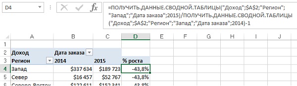
After you finish copying the formula, glancing at the screen, you will realize that something is wrong - each region has shown a drop of 43.8% over the year (Fig. 3).

Figure: 3. When you finish copying the formula to all cells in the column, you will see that each region showed a 43.8% drop

This is unlikely to happen in real life. Anyone will tell you that after following the steps above, Excel will create the formula \u003d C4 / B4-1. Go back to cell D4 and notice the formula bar (Figure 4). Just some devilry! The simple formula \u003d C4 / B4-1 no longer exists. Instead of it, the program substitutes a complex construction with the GET.DATA.PUMP.TABLE function. Why does this formula give correct results in cell D4, but after copying to the cells below it refuses to work?

The first reaction of any user to what happened will be the following: "What is this strange GET.DATA.PERSONAL.TABLE construction that ruined my report?" Most users will want to get rid of this feature right away. Some will ask the question, "Why did Microsoft slip this feature to us?"

There was nothing like this in excel times 2000. Having started to regularly encounter the GET.DATA.PERSONAL.TABLES function, I just hated it. When at one of the seminars someone asked me how it could be used for the good of the cause, I was dumbfounded. I have never asked myself such a question! In my opinion, and in the opinion of most Excel users, the GET.DATA.PUMP.TABLE function was a product of evil that had nothing to do with the forces of good. Fortunately, there are two ways to disable this feature.

Blocking the GET PIVOTTABLE DATA function by entering a formula.There is a simple way to prevent the GET PIVOTTABLE function from appearing. To do this, you need to create a formula without using the mouse or cursor keys. Just follow these steps.

Go to cell D4 and type \u003d (equal sign).
Enter C4.
Enter a / (forward slash for division).
Enter B4.
Enter -1.
Click Enter.

You have now created a regular excel formula, which can be copied to the cells below the column and with which you can get the correct results (Fig. 5). As you can see, you can create formulas in areas outside the PivotTable that refer to data within the PivotTable. And those who do not believe that this is possible, let them perform the described actions on their own.

Figure: 5. Just enter \u003d C4 / B4-1 from the keyboard, and the formula will work as you need

Some users will feel uncomfortable with the usual order of entering formulas. In addition, the proposed option is more laborious. If you are one of these users, the second way is for you ...

Disable the GET PANEL.TABLE DATA function.You can permanently disable the GET PANEL.TABLE DATA function. Click on the menu ribbon File → Options... In the opened window OptionsExcel go to contribution Formulas and uncheck the box next to the option Use functionGetPivotData for Pivot Table Links... Click Ok.

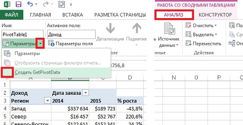
Alternative option. Click on the pivot table, and in the contextual tab that appears Analysis click on the drop-down list next to the button Options... Uncheck the box next to Create GetPivotData (fig. 7). The checkbox is on by default.

Why did Microsoft offer us the GET PANEL.TABLES feature.If this feature is so awful, why did Microsoft enable it by default? Why do they care about maintaining support for this feature in newer versions of Excel? Are they aware of user sentiment? And we move on to the fun part ...

Using GET PIVOTTABLE DATA to Improve PivotTables

Pivot tables are a great invention of humanity. The pivot table is created with just a few clicks, eliminating the need to apply advanced filter, BDSUMM function and data tables. With pivot tables, you can create one-page reports from huge amounts of data. These advantages overshadow some of the disadvantages of pivot tables, such as lackluster formatting and the need to convert pivot tables to values \u200b\u200bfor additional customization. In fig. Figure 8 shows a typical process for creating a pivot table. In this case, everything starts with the initial data. We create a pivot table and use all possible techniques to customize and improve it. Sometimes we convert the pivot table to values \u200b\u200band do some final formatting.

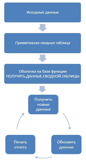
The new PivotTable methodology proposed by Rob Colley (a developer at Microsoft) and discussed below is the result of improvements to the process described above. In this case, a primitive pivot table is created first. This table does not need to be formatted. A one-step, relatively time-consuming process is then followed to create a nicely formatted shell that will house the final report. After that, the GET.DATA.PERSONAL.TABLE function is used to quickly fill a report that is in the shell with data. After receiving the new data, you can put it on the sheet, update the primitive pivot table and print the report that is in the shell (Figure 9). This technique has a number of undeniable advantages. For example, you don't have to worry about formatting your report immediately after you create it. The process of creating pivot tables becomes almost completely automated.

The following sections discuss how to create a dynamic report that displays actual figures for past months and targets for future months.

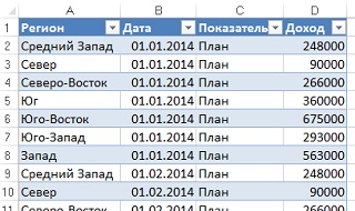
Create a primitive pivot table.Initial data (Fig. 10) are presented in the form of transactions containing information on planned and actual indicators for each region in which there are branches of the company. Planned figures are detailed at the month level, and actual figures at the level of individual days. Planned indicators are created for the year ahead, and actual indicators are created for the past months. Since the report will be updated every month, this process is greatly simplified if the data source of the PivotTable grows in size as new data is added to the bottom. In outdated versions Excel creation a similar data source was implemented using a named dynamic range using the OFFSET function (see details). When working in Excel 2013, simply select one of the data cells, and press the key combination Ctrl + T (create a Table). This will create a named dataset that automatically expands as new rows and columns are added.

Now let's create a pivot table. The GET.PIVOTTABLE function is powerful enough, but it can only return the values \u200b\u200bthat appear in the current PivotTable. This function is unable to perform a cache scan to calculate items that are not in the pivot table.

Create a pivot table:

Select Team Insert → Pivot tableand then in the dialog Creating a pivot tableclick OK.
In the PivotTable Field List, select a field date... A list of dates will appear on the left side of the pivot table (Fig. 11).
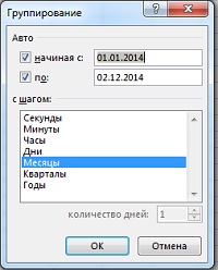
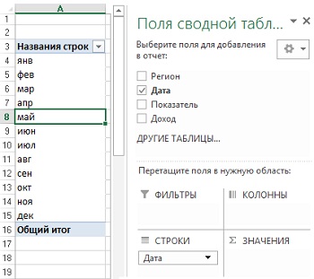
Select any date cell, for example A4. On the contextual tab Analysislocated in the set of contextual tabs Working with pivot tables, click the button Grouping by field (see details). In the dialog box Grouping select an option Months (fig. 12). Click OK... The names of the months will appear on the left side of the pivot table (Fig. 13).
Drag the field date to the Columns area of \u200b\u200bthe PivotTable.
Drag the field Index to the Columns area of \u200b\u200bthe PivotTable Field List.
Select a field Regionto be displayed in the left column of the pivot table.
Select a field Incomethat appears in the PivotTable Values \u200b\u200barea.

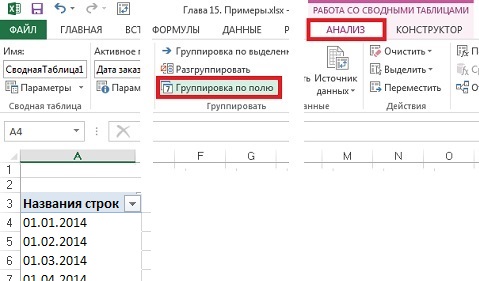
Figure: 11. Start by grouping by field date

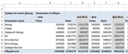
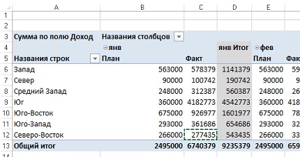
At this point, our pivot table looks pretty primitive (Figure 14). I really don't like lettering Line names and Column names... It is impractical to display totals for Jan Plan and Jan Fact in column D, etc. But don't worry about appearance this pivot table, because, besides you, no one else will see it. From this point on, we will create a report wrapper, the data source for which will be the newly created pivot table.

Creation of the report shell.Insert a blank sheet into your workbook. Let's put aside the PivotTable tools for a while and move on to regular Excel tools. Our task is to use formulas and formatting to create a beautiful report that is not ashamed to show to the manager.

Proceed as follows (fig. 15).

In cell A1, enter the name of the report - Planned and actual indicators by region.
Go to the tab home, click on the button Cell Styles select format Heading 1.
In cell A2, enter the formula \u003d EON MONTHS (TODAY (); 0). This function returns the last day of the current month. For example, if you read these lines on August 14, 2014, cell A2 will display the date August 31, 2014.
Select cell A2. Press the key combination Ctrl + 1 to display the dialog box Cell format... In the tab Number click on item All formats... Enter a custom number format as "From the month" MMMM "planned indicators" (fig. 16). As a result, the calculated date will look like text.
In cell A5 enter a title Region.
Enter the region headings in the remaining cells in column A. The region headings must match the region names shown in the pivot table.
Add labels to the column for totals by department, if necessary.
At the bottom of the report add the line Total for the company.
In cell B4, enter the formula \u003d DATE (YEAR ($ A $ 2); COLUMN (A1); 1). This formula returns the dates 01/01/2014, 01/02/2104, etc., the first days of all 12 months of the current year.
Select cell B4. Press the key combination Ctrl + 1 to open the window Cell format... In the tab Number in section All formats enter a custom number format Mmm... This format displays the three-letter month name. Align the text to the right of the cell.
Copy the contents of cell B4 to the range C4: M4. A row with the names of the months appears at the top of the pivot table.
In cell B5, enter the formula \u003d IF (MONTH (B4)<МЕСЯЦ($A$2); " Факт " ; " План "). Содержимое ячейки В5 выровняйте по правому краю. Скопируйте это содержимое в диапазон ячеек С5:М5. В результате для прошедших месяцев будет отображаться слово Fact, and for the current and future - Plan.
Add a title to cell N5 Outcome... To cell O4 - Outcome, O5 - Plan, P5 - % deviation.
Enter the usual Excel formulas used to calculate department totals, company total row, grand total column, and% variance column:
1. in cell B8, enter the formula \u003d SUM (B6: B7) and copy it to other cells in the row;
2. in cell N6, enter the formula \u003d SUM (B6: M6) and copy it to other cells in the column;
3. in cell P6, enter the formula \u003d IFERROR ((N6 / O10) -1; 0) and copy it to other cells in the column;
4. in cell B13, enter the formula \u003d SUM (B10: B12) and copy it to other cells in the row;
5. in cell B17 enter the formula \u003d SUM (B15: B16) and copy it to other cells in the row;
6. in cell B19 enter the formula \u003d SUM (B6: B18) / 2 and copy it to other cells in the row.
Apply the Heading 4 style to the labels in column A and to the headings in rows 4 and 5.
For the range of cells B6: O19, select the number format # ## 0.
For the cells in column P, select the number format 0.0%.

So, we have completed the creation of the report shell shown in Fig. 15. This report includes all required formatting. The next section demonstrates how to use the GET PIVOTTABLE DATA function to complete a report.

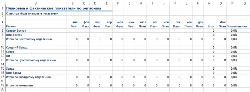
Figure: 15. Report wrapper before adding formulas GET.DATA.PERSONAL.TABLES

Using the GET PIVOTTABLE DATA function to populate the report shell with data.From now on, you will be able to experience all the benefits of using the GET PANEL.TABLE DATA function. If you have cleared the checkbox enabling this function, return to the corresponding setting and return the checkbox (see description in Fig. 6 or 7).

Select cell B6 of the report shell. This cell corresponds to the North East region and actual figures for January.

Enter \u003d (equal sign) to start entering the formula.
Go to the sheet from the pivot table and click on the cell that corresponds to the northeast region and the actual figures for January - C12 (Fig. 17).
Press the key Enterto finish entering the formula and return to the report shell. As a result, Excel will add the function GET PIVOTTABLE DATA in cell B6. The cell will display the value of $ 277,435.

Remember this number, as it will be required when comparing with the results of the formula, which you will edit later. The formula generated by the program has the following form: \u003d GET.DATA.PUMP.TABLE ("Income"; 'Fig. 11-14 ′! $ A $ 3; "Region"; "North-East"; "Date"; 1; "Indicator"; "Fact"). If you've ignored the GET PivotTable function so far, it's time to take a closer look. In fig. 18 this formula is shown in edit mode along with a hint.

Function arguments:

Data_field. A field from the value area of \u200b\u200bthe pivot table. Please note: in this case, the field is used Income, but not Amount in the Income field.
Pivot_table. With this parameter, Microsoft asks you, "Which pivot table do you want to use?" It is enough to specify one of the pivot table cells. The entry 'Fig. 11-14 '! $ A $ 3 refers to the first cell of the PivotTable where data is entered. Since in our case, you can specify any cell related to the pivot table, leave the argument unchanged. Cell address $ A $ 3 is suitable in all respects.
Field 1; element 1. In the automatically generated formula, the name of the field is selected Region, and as the field value - Northeast... This is where the reason for the problems that arise when working with the GET DATA.PUMP.TABLE function lies. Autoselected values \u200b\u200bcannot be copied because they are hardcoded. Therefore, if you copy formulas in the entire report area, you will have to change them manually. Replace Northeast with a cell reference of the form $ A6. By placing a dollar sign in front of Column A, you determine whether the row portion of the reference can be changed when you copy the formula into the cells in the column.
Field 2; item 2. This pair of arguments defines the field date with a value of 1. If the original PivotTable was grouped by month, the month field retains the original field name date... The numeric value of the month is 1, which corresponds to January. It is hardly advisable to use such a value when creating huge formulas that are specified in dozens or even hundreds of report cells. Better to use a formula that calculates the field values date, like the formula in cell B4. Instead of 1 in this case, you can use the formula MONTH (In $ 4). The dollar sign preceding the 4 indicates that the formula can assign values \u200b\u200bto the field date based on other months as the formula is copied into the cells in the row.
Field 3; element 3. In this case, the field name is automatically assigned Index and field value Fact... These values \u200b\u200bare correct for January, but for subsequent months the field value will have to be changed to Plan. Change the hard-coded value of the field Fact to the link B $ 5.
Field 4; Element 4. These arguments are not used because the fields are over.

The new formula is shown in Fig. 19. In a minute, instead of a hard-coded formula designed to work with a single value, a flexible formula was created that can be copied to all cells in the dataset. Press the key Enterand you will get the same result as before editing the formula. The edited formula takes the following form: \u003d GET.PUMP.TABLE DATA ("Income"; 'Fig. 11-14 ′! $ A $ 3; "Region"; $ A6; "Date"; MONTH (B $ 4); "Indicator "; B $ 5)

Figure: 19. Upon completion of editing, the formula GET.DATA.PUMP.TABLE is suitable for copying to all cells of the range

Copy the formula to any blank cells in columns B: M where the results are calculated. Now that the report contains real numbers, you can make final adjustments to the column widths.

In the next step, we will set up the GET.PUMP.TABLE formula to calculate the final targets. If you just copy the formula into cell O6, the error message #REF! The reason for this error is that the word Outcome in cell O4 is not the month name. To ensure the correct operation of the GET PIVOTTABLE DATA function, the required value must be in the PivotTable. But since in the original pivot table, the field Index is the second field in the column area, the data column Plan summary actually absent. Move the field Index so that it becomes the first in the column area (Figure 20).

Figure: 20. Adjust the layout of the fields in the column area so that the column appears Outline plan

Compare with fig. 14. There, in the area of \u200b\u200bthe COLUMN, the field was the first date, which led to the fact that at first the columns were grouped by date, and within each month by plan / fact. Now the first is the Indicator field, and in the summary, columns are first Plan, internally sorted by month and then all columns Fact.

Returning to the sheet of the report envelope, stand in cell O6, type \u003d (equal sign) and refer to cell N12 on the sheet of the pivot table, corresponding to the planned results of the Northeast region. Click Enter... The result is the formula \u003d GET.DATA.PERSONAL.TABLES ("Income"; "Fig. 11-14"! $ A $ 3; "Region"; "North-East"; "Indicator"; "Plan"). Edit it: \u003d GET. DATA.SUMMARY.TABLES ("Income"; ’Fig. 11-14 ′! $ A $ 3;" Region "; $ A6;" Indicator "; O $ 5). Copy this formula to other cells in column O (Figure 21). Please note that even if you move different areas of the PivotTable report, the shell works correctly. Of course, if you make some pivot fields inactive, the shell will not cope with this ...

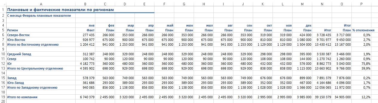
Figure: 21. Final report that can be presented to the manager

You now have a well-formatted report wrapper that uses values \u200b\u200bfrom a dynamic PivotTable. Although the initial creation of the report took quite a long time, updating it took only a few minutes.

Refreshing the report.To update the report with data for future months, follow these steps.

Insert actual figures below the original dataset. Because the source data is in a table format, table formatting is automatically propagated to new data rows. It also expands the definition of the original PivotTable (in the Excel file, I already added the actual figures for the whole year).
Go to the pivot table. Right click and select Refresh... The look of the pivot table will change, but that's okay.
Go to the report shell. In principle, everything has already been done to update the report, but it doesn't hurt to test the results. Change the formula in cell A2, for example, to this: \u003d EON MONTHS (TODAY () +31 ; 0), and see what happens.

By adding new actual sales data every month, you don't have to worry about re-creating formats, formulas, etc. The described process of updating the report is so simple that you will forget about the problems that arose during the preparation of monthly reports forever. The only problem can arise if the company is reorganized, as a result of which new regions may appear in the pivot table. To ensure that the formulas work correctly, check that the grand total in your report matches the total in the pivot table. When a new region appears, just add it to the wrapped sheet and drag the appropriate formulas.

I didn't think I would ever say the following: “The GET.DATA.PUMP.TABLE function is the greatest blessing. How did we exist without her before? "

In the original, Jelena's initial data was arranged so that further formulas worked correctly only in July 2015.In the Excel file attached to this note, I modified the original data, as well as some formulas so that everything worked, regardless of the date when you you will experiment with the attached Excel file. Unfortunately, the formulas had to be complicated.

Earlier I already talked about the fact that when referencing a pivot table cell, instead of a normal link, the GET.PIVOTTABLE DATA function is returned (see). If you are interested in as to overcome this inconvenience, I recommend referring to the mentioned note. If you're wondering, why this is how it happens, and also what are the positive aspects of the function GET DATA.COMPLETE.TABLE, then I suggest a fragment of the book Jelen, Alexander. (chapter 15). The technique under consideration will allow you to cope with many problems that cause headaches for users of pivot tables, in particular:

When the PivotTable is refreshed, the previously applied formatting disappears. Number formats are lost. Column width adjustment results disappear.
There is no easy way to create an asymmetric PivotTable. The only option is to use named sets, but this method is only available to those using Data Model Pivot Tables and not regular Pivot Tables.
Excel cannot remember templates. If you need to re-create PivotTables over and over again, you will have to re-group, apply calculated fields and members, and perform a number of other similar tasks.

Download a note in format or, examples in format

Well, let's start in order.

How to abandon the problematic function GET DATA.PERSONAL TABLES

Suppose in the pivot table shown in Fig. 1, you need to compare the data for 2015 and 2014.

Figure: 1. Original pivot table

Add the heading "% Height" to cell D3.
Copy the format from cell C3 to cell D3.
Enter an equal sign in cell D4.
Click on cell C4.
Enter the / (forward slash) sign to represent the division operation.
Click on cell B4.
Enter -1 and press the key combination to stay in the same cell. Format the result as a percentage. You will see that the West region experienced a 43.8% drop in income (Figure 2). Not very good results.
When you finish entering your first formula, select cell D4.
Double click on the small square located in the lower right corner of the cell. This square represents a fill handle that you can use to copy a formula to fill an entire column in the report.

After you finish copying the formula, glancing at the screen, you will realize that something is wrong - each region has shown a drop of 43.8% over the year (Fig. 3).

Figure: 3. When you finish copying the formula to all cells in the column, you will see that each region showed a 43.8% drop

Nothing like this happened in the days of Excel 2000. When I started to regularly encounter the GETDATA.PERSONAL.TABLES function, I just hated it. When at one of the seminars someone asked me how it could be used for the good of the cause, I was dumbfounded. I have never asked such a question! In my opinion, and in the opinion of most Excel users, the GET.DATA.PUMP.TABLE function was a product of evil that had nothing to do with the forces of good. Fortunately, there are two ways to disable this feature.

Go to cell D4 and type \u003d (equal sign).
Enter C4.
Enter a / (forward slash for division).
Enter B4.
Enter -1.
Click Enter.

Now you have created a regular Excel formula that you can copy into the cells below the column and with which you can get the correct results (Figure 5). As you can see, you can create formulas in areas outside the PivotTable that refer to data within the PivotTable. And those who do not believe that this is possible, let them perform the described actions on their own.

Figure: 5. Just enter \u003d C4 / B4-1 from the keyboard, and the formula will work as you need

Some users will feel uncomfortable with the usual order of entering formulas. In addition, the proposed option is more laborious. If you are one of these users, the second way is for you ...

Using GET PIVOTTABLE DATA to Improve PivotTables

The following sections discuss how to create a dynamic report that displays actual figures for past months and targets for future months.

Create a primitive pivot table.Initial data (Fig. 10) are presented in the form of transactions containing information about planned and actual indicators for each region in which there are branches of the company. Planned figures are detailed at the month level, and actual figures at the level of individual days. Planned indicators are created for the year ahead, and actual indicators are created for the past months. Since the report will be updated every month, this process is greatly simplified if the data source of the PivotTable grows in size as new data is added to the bottom. In older versions of Excel, such a data source was created using a named dynamic range using the OFFSET function (see details). When working in Excel 2013, simply select one of the data cells, and press the key combination Ctrl + T (create a Table). This will create a named dataset that automatically expands as new rows and columns are added.

Create a pivot table:

Select Team Insert → Pivot tableand then in the dialog Creating a pivot tableclick OK.
In the PivotTable Field List, select a field date... A list of dates will appear on the left side of the pivot table (Fig. 11).
Select any date cell, for example A4. On the contextual tab Analysislocated in the set of contextual tabs Working with pivot tables, click the button Grouping by field (see details). In the dialog box Grouping select an option Months (fig. 12). Click OK... The names of the months will appear on the left side of the pivot table (Fig. 13).
Drag the field date to the Columns area of \u200b\u200bthe PivotTable.
Drag the field Index to the Columns area of \u200b\u200bthe PivotTable Field List.
Select a field Regionto be displayed in the left column of the pivot table.
Select a field Incomethat appears in the PivotTable Values \u200b\u200barea.

Figure: 11. Start by grouping by field date

At this point, our pivot table looks pretty primitive (Figure 14). I really don't like lettering Line names and Column names... It is impractical to display totals for Jan Plan and Jan Fact in column D, etc. But don't worry about the look of this pivot table, because no one else will see it except you. From this point on, we will be creating a report shell, the data source for which will be the newly created pivot table.

Proceed as follows (fig. 15).

In cell A1, enter the name of the report - Planned and actual indicators by region.
Go to the tab home, click on the button Cell Styles select format Heading 1.
In cell A2, enter the formula \u003d EON MONTHS (TODAY (); 0). This function returns the last day of the current month. For example, if you read these lines on August 14, 2014, cell A2 will display the date August 31, 2014.
Select cell A2. Press the key combination Ctrl + 1 to display the dialog box Cell format... In the tab Number click on item All formats... Enter a custom number format as "From the month" MMMM "planned indicators" (fig. 16). As a result, the calculated date will look like text.
In cell A5 enter a title Region.
Enter the region headings in the remaining cells in column A. The region headings must match the region names shown in the pivot table.
Add labels to the column for totals by department, if necessary.
At the bottom of the report add the line Total for the company.
In cell B4, enter the formula \u003d DATE (YEAR ($ A $ 2); COLUMN (A1); 1). This formula returns the dates 01/01/2014, 01/02/2104, etc., the first days of all 12 months of the current year.
Select cell B4. Press the key combination Ctrl + 1 to open the window Cell format... In the tab Number in section All formats enter a custom number format Mmm... This format displays the three-letter month name. Align the text to the right of the cell.
Copy the contents of cell B4 to the range C4: M4. A row with the names of the months appears at the top of the pivot table.
In cell B5, enter the formula \u003d IF (MONTH (B4)<МЕСЯЦ($A$2); " Факт " ; " План "). Содержимое ячейки В5 выровняйте по правому краю. Скопируйте это содержимое в диапазон ячеек С5:М5. В результате для прошедших месяцев будет отображаться слово Fact, and for the current and future - Plan.
Add a title to cell N5 Outcome... To cell O4 - Outcome, O5 - Plan, P5 - % deviation.
Enter the usual Excel formulas used to calculate department totals, company total row, grand total column, and% variance column:
1. in cell B8, enter the formula \u003d SUM (B6: B7) and copy it to other cells in the row;
2. in cell N6, enter the formula \u003d SUM (B6: M6) and copy it to other cells in the column;
3. in cell P6, enter the formula \u003d IFERROR ((N6 / O10) -1; 0) and copy it to other cells in the column;
4. in cell B13, enter the formula \u003d SUM (B10: B12) and copy it to other cells in the row;
5. in cell B17 enter the formula \u003d SUM (B15: B16) and copy it to other cells in the row;
6. in cell B19 enter the formula \u003d SUM (B6: B18) / 2 and copy it to other cells in the row.
Apply the Heading 4 style to the labels in column A and to the headings in rows 4 and 5.
For the range of cells B6: O19, select the number format # ## 0.
For the cells in column P, select the number format 0.0%.

Figure: 15. Report wrapper before adding formulas GET.DATA.PERSONAL.TABLES

Select cell B6 of the report shell. This cell corresponds to the North East region and actual figures for January.

Enter \u003d (equal sign) to start entering the formula.
Go to the sheet from the pivot table and click on the cell that corresponds to the northeast region and the actual figures for January - C12 (Fig. 17).
Press the key Enterto finish entering the formula and return to the report shell. As a result, Excel will add the function GET PIVOTTABLE DATA in cell B6. The cell will display the value of $ 277,435.

Function arguments:

Data_field. A field from the value area of \u200b\u200bthe pivot table. Please note: in this case, the field is used Income, but not Amount in the Income field.
Pivot_table. With this parameter, Microsoft asks you, "Which pivot table do you want to use?" It is enough to specify one of the pivot table cells. The entry 'Fig. 11-14 '! $ A $ 3 refers to the first cell of the PivotTable where data is entered. Since in our case, you can specify any cell related to the pivot table, leave the argument unchanged. Cell address $ A $ 3 is suitable in all respects.
Field 1; element 1. In the automatically generated formula, the name of the field is selected Region, and as the field value - Northeast... This is where the reason for the problems that arise when working with the GET DATA.PUMP.TABLE function lies. Autoselected values \u200b\u200bcannot be copied because they are hardcoded. Therefore, if you copy formulas in the entire report area, you will have to change them manually. Replace Northeast with a cell reference of the form $ A6. By placing a dollar sign in front of Column A, you determine whether the row portion of the reference can be changed when you copy the formula into the cells in the column.
Field 2; item 2. This pair of arguments defines the field date with a value of 1. If the original PivotTable was grouped by month, the month field retains the original field name date... The numeric value of the month is 1, which corresponds to January. It is hardly advisable to use such a value when creating huge formulas that are specified in dozens or even hundreds of report cells. Better to use a formula that calculates the field values date, like the formula in cell B4. Instead of 1 in this case, you can use the formula MONTH (In $ 4). The dollar sign preceding the 4 indicates that the formula can assign values \u200b\u200bto the field date based on other months as the formula is copied into the cells in the row.
Field 3; element 3. In this case, the field name is automatically assigned Index and field value Fact... These values \u200b\u200bare correct for January, but for subsequent months the field value will have to be changed to Plan. Change the hard-coded value of the field Fact to the link B $ 5.
Field 4; Element 4. These arguments are not used because the fields are over.

Figure: 19. Upon completion of editing, the formula GET.DATA.PUMP.TABLE is suitable for copying to all cells of the range

Copy the formula to any blank cells in columns B: M where the results are calculated. Now that the report contains real numbers, you can make final adjustments to the column widths.

Figure: 20. Adjust the layout of the fields in the column area so that the column appears Outline plan

Figure: 21. Final report that can be presented to the manager

Refreshing the report.To update the report with data for future months, follow these steps.

Insert actual figures below the original dataset. Because the source data is in a table format, table formatting is automatically propagated to new data rows. It also expands the definition of the original PivotTable (in the Excel file, I already added the actual figures for the whole year).
Go to the pivot table. Right click and select Refresh... The look of the pivot table will change, but that's okay.
Go to the report shell. In principle, everything has already been done to update the report, but it doesn't hurt to test the results. Change the formula in cell A2, for example, to this: \u003d EON MONTHS (TODAY () +31 ; 0), and see what happens.

I didn't think I would ever say the following: “The GET.DATA.PUMP.TABLE function is the greatest blessing. How did we exist without her before? "

For pivot tables, the GET.DATA.PIVOTTABLE function is a function that returns the data stored in the pivot table report.

To get quick access to the function, you need to enter an equal sign in the cell (\u003d) and select the required cell in the pivot table. Excel will generate the GET PIVOTTABLE DATA function automatically.

Disable GetPivotData creation

To turn off the automatic generation of the GET PIVOTTABLE function, select any cell in the pivot table, click the tab Working with pivot tables -\u003e Optionsto the group Pivot table.Click the down arrow next to the tab Options.In the drop-down menu, uncheck the box Create aGetPivotData.

Using Cell References in the GET DATA.PUMP.TABLE function

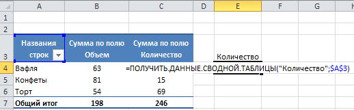
Instead of specifying the names of items or fields in the GET.PUMP.TABLE function, you can refer to cells on the sheet. In the example below, cell E3 contains the product name, and the formula in cell E4 refers to it. As a result, the total volume for the cakes will be returned.

Using PivotTable Field References

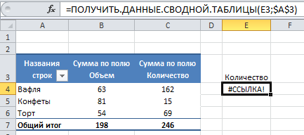
There are no questions about how links to pivot table items work; problems arise if we want to refer to a data field.

In the example, cell E3 contains the data field name "Quantity", and it would be nice to reference this cell in the function, instead of having the field name in the GET.DATA.PUMP.TABLE formula.

However, if we change the first argument data_fieldto the reference to cell E3, Excel will return us the error #REF!

GET.PERSONAL.TABLE DATA (E3; $ A $ 3)

The problem is solved simply by adding an empty string (“”) to the beginning or end of the cell reference.

GET.PERSONAL.TABLE DATA (E3 & ""; $ A $ 3)

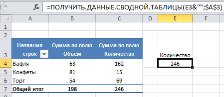
A simple correction to the formula will return the correct value.

Using dates in the GET.DATA.PUMP.TABLE function

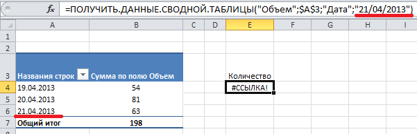
If you use dates in the GET PIVOTTABLE DATA function, you may have problems even if the date is displayed in the PivotTable. For example, the formula below is the date “04/21/2013” \u200b\u200band the pivot table contains a field with sales dates. However, the formula in cell E4 returns an error.

GET.DATA.PERSONAL.TABLE ("Volume"; $ A $ 3; "Date"; "04/21/2013")

To avoid errors related to dates, you can use one of the following methods:

Compare Date Formats in Formula and Pivot Table
Use DATEVALUE function
Use the DATE function
Refer to cell with correct date

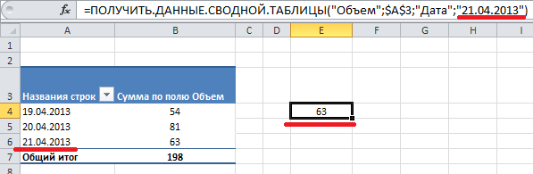
Compare date formats in formula and PivotTable.

To get the correct result, when using the GET PIVOTTABLE DATA function, make sure that the date formats of the formula argument and the PivotTable are the same.

In cell E4, the formula uses the date format “DD.MM.YYYY” and returns the correct information as a result.

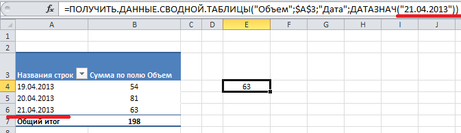
Using the DATEVALUE function

Instead of manually entering the date in the formula, you can add the DATEVALUE function to return the date.

In cell E4, the date is entered using the DATEVALUE function, and Excel returns the required information.

RECEIVE.SUMMARY.TABLE.DATA ("Volume"; $ A $ 3; "Date"; DATEVALUE ("04.21.2013"))

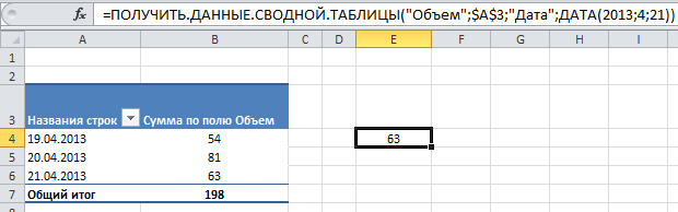
Using the DATE function

Instead of manually entering the date in the formula, you can use the DATE function, which will allow you to correctly return the necessary information.

RECEIVE.SUMMARY.TABLE.DATA ("Volume"; $ A $ 3; "Date"; DATE (2013; 4; 21))

Date cell reference

Instead of manually entering a date in a formula, you can reference a cell that contains a date (in any format that Excel interprets data as dates). In the example in cell E4, the formula refers to cell E3 and Excel returns the correct data.

GET.DATA.COMPLETE.TABLE ("Volume"; $ A $ 3; "Date"; E3)