Using a boolean function if examples. Microsoft Excel Feature: Finding a Solution
Solving nonlinear equations and systems "
Objective: Exploring the capabilities of Ms Excel 2007 in solving nonlinear equations and systems. Acquisition of skills in solving nonlinear equations and systems using the package.
Exercise 1. Find the roots of the polynomial x 3 - 0.01x 2 - 0.7044x + 0.139104 \u003d 0.
First, let's solve the equation graphically. It is known that the graphical solution of the equation f (x) \u003d 0 is the point of intersection of the graph of the function f (x) with the abscissa, i.e. such a value of x at which the function vanishes.
Let's tabulate our polynomial on the interval from -1 to 1 with a step of 0.2. The calculation results are shown in Fig., Where the formula was entered into cell B2: \u003d A2 ^ 3 - 0.01 * A2 ^ 2 - 0.7044 * A2 + 0.139104. The graph shows that the function crosses the Ox axis three times, and since the third degree polynomial has no more than three real roots, a graphical solution to the problem has been found. In other words, the roots were localized, i.e. the intervals on which the roots of this polynomial are located are determined: [-1, -0.8], and.
Now you can find the roots of the polynomial by successive approximations using the command Data → Working with data → What-If analysis → Parameter selection.
After entering the initial approximations and values \u200b\u200bof the function, you can turn to the command Data → Working with data → What-If analysis → Parameter selection and populate the dialog as follows.
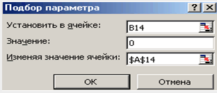
In field Set in cella reference is given to the cell in which the formula is entered that calculates the value of the left side of the equation (the equation must be written so that its right side does not contain a variable). In field Value we enter the right side of the equation, and in the field Changing cell values a reference to the cell allocated for the variable is given. Note that entering cell references in the fields of the dialog Selection of parameters it is more convenient not from the keyboard, but by clicking on the corresponding cell.
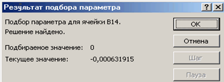
After pressing the OK button, the Result of parameter selection dialog box appears with a message about the successful completion of the search for a solution, the approximate value of the root will be placed in cell A14.
Find the two remaining roots in the same way. The calculation results will be placed in cells A15 and A16.

Task 2. Solve the equation e x - (2x - 1) 2 = 0.
Let's localize the roots of the nonlinear equation.
To do this, we represent it in the form f (x) \u003d g (x), i.e. e x \u003d (2x - 1) 2 or f (x) \u003d e x, g (x) \u003d (2x - 1) 2, and solve graphically.
The graphical solution to the equation f (x) \u003d g (x) will be the intersection point of the lines f (x) and g (x).
Let's build graphs f (x) and g (x). To do this, enter the values \u200b\u200bof the argument into the range A3: A18. In cell B3 we enter the formula for calculating the values \u200b\u200bof the function f (x): \u003d EXP (A3), and in C3 for calculating g (x): \u003d (2 * A3-1) ^ 2.
Calculation results and plotting f (x) and g (x):
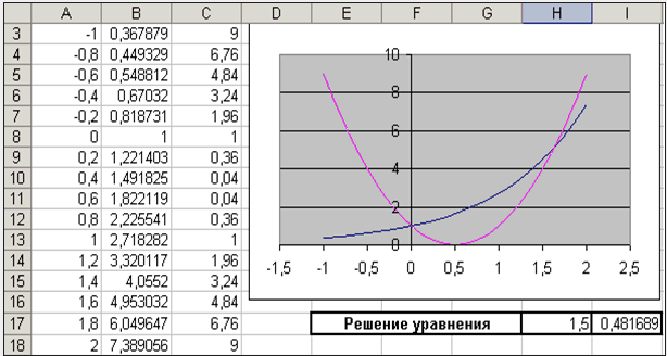
The graph shows that the lines f (x) and g (x) intersect twice, i.e. this equation has two solutions. One of them is trivial and can be calculated exactly:

For the second, the root isolation interval can be determined: 1.5< x < 2.
Now you can find the root of the equation on a segment by the method of successive approximations.
Let's enter the initial approximation into cell H17 \u003d 1.5, and the equation itself, with reference to the initial approximation, into cell I17 \u003d EXP (H17) - (2 * H17-1) ^ 2.
and fill in the dialog box Parameter selection.
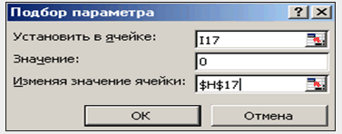
The result of the search for a solution will be displayed in cell H17.
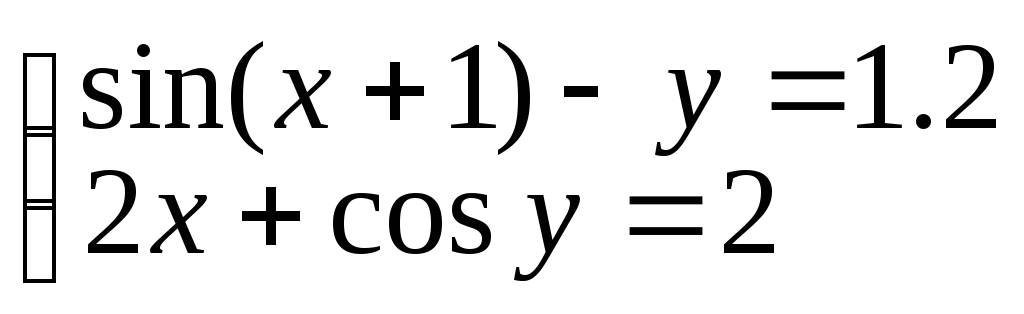
The task3 . Solve the system of equations:
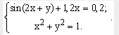
Before using the methods described above for solving systems of equations, we will find a graphical solution to this system. Note that both equations of the system are given implicitly and to construct graphs corresponding to these equations, it is necessary to solve the given equations with respect to the variable y.
For the first equation of the system, we have:
Let's find out the ODV of the resulting function:
The second equation of this system describes a circle.
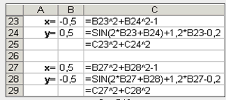
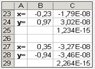
Fragment of MS Excel worksheet with formulas that must be entered into cells to build lines described by the equations of the system. The intersection points of the lines depicted are a graphical solution to a system of nonlinear equations.

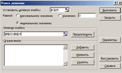
It is not difficult to see that the given system has two solutions. Therefore, the procedure for finding solutions to the system must be performed twice, having previously determined the root isolation interval along the Ox and Oy axes. In our case, the first root lies in the intervals (-0.5; 0) x and (0.5; 1) y, and the second one is (0; 0.5) x and (-0.5; -1) y. We will proceed as follows. Let us introduce the initial values \u200b\u200bof the variables x and y, formulas representing the equations of the system and the goal function.
Now we will use the command Data → Analysis → Search for solutions twice, filling in the dialog boxes that appear.
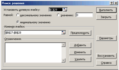
Comparing the obtained solution of the system with the graphical one, we make sure that the system is solved correctly.
Self-help assignments
Exercise 1... Find the roots of a polynomial
Assignment 2... Find the solution to the nonlinear equation.

Assignment 3... Find the solution to a system of nonlinear equations.
As you already know, the formulas in Microsoft Excel allow you to determine the value of a function by its arguments. However, a situation may arise when the value of the function is known, and the argument needs to be found (i.e., to solve the equation). To solve such problems, there is a special function Goal Seek .
Parameter search.
Special function Goal Seek allows you to define a parameter (argument) of a function if its value is known. When a parameter is selected, the value of the influencing cell (parameter) is changed until the formula that depends on this cell returns the specified value.
 Let us consider the procedure for finding a parameter using a simple example: solve the equation 10 * x - 10 / x \u003d 15
... Here parameter (argument) - x
... Let it be a cell A3
... Let's enter in this cell any number that lies in the scope of the function definition (in our example, this number cannot be equal to zero). This value will be used as the starting value. Let it be 3
... We introduce the formula \u003d 10 * A3-10 / A3
, by which the required value should be obtained, into some cell, for example, B3
... Now you can start the parameter search function by selecting the command Goal Seek
on the menu Tools
... Enter search parameters:
Let us consider the procedure for finding a parameter using a simple example: solve the equation 10 * x - 10 / x \u003d 15
... Here parameter (argument) - x
... Let it be a cell A3
... Let's enter in this cell any number that lies in the scope of the function definition (in our example, this number cannot be equal to zero). This value will be used as the starting value. Let it be 3
... We introduce the formula \u003d 10 * A3-10 / A3
, by which the required value should be obtained, into some cell, for example, B3
... Now you can start the parameter search function by selecting the command Goal Seek
on the menu Tools
... Enter search parameters:
- In field Set cell enter a reference to the cell containing the formula you want.
- Enter the search result in the field To value .
- In field By changing cell enter a reference to the cell containing the value to be matched.
- Click on the key OK .
 At the end of the function, a window will appear on the screen in which the search results will be displayed. The found parameter will appear in the cell that was reserved for it. Pay attention to the fact that in our example the equation has two solutions, and the parameter is matched only one - this is because the parameter changes only until the required value is returned. The first argument found in this way is returned to us as a search result. If we specify as the initial value in our example -3
, then the second solution to the equation will be found: -0,5
.
At the end of the function, a window will appear on the screen in which the search results will be displayed. The found parameter will appear in the cell that was reserved for it. Pay attention to the fact that in our example the equation has two solutions, and the parameter is matched only one - this is because the parameter changes only until the required value is returned. The first argument found in this way is returned to us as a search result. If we specify as the initial value in our example -3
, then the second solution to the equation will be found: -0,5
.
It is rather difficult to correctly determine the most suitable starting value. More often we can make some assumptions about the desired parameter, for example, the parameter must be integer (then we get the first solution to our equation) or non-positive (the second solution).
The task of finding a parameter with imposed boundary conditions will be helped by a special add-in Microsoft Excel Solver .
Search for a solution.
Microsoft Excel add-in Solver is not automatically installed in a typical installation:
- On the menu Tools select team Add-Ins ... If the dialog box Add-Ins does not contain command Solver , press the button Browse and specify the drive and folder that contains the add-in file Solver.xla (usually this is the folder Library \\ Solver ) or run the program microsoft installations Office if it can't find the file.
- In the dialog box Add-Ins check the box Solver .
The procedure for finding a solution allows you to find the optimal value of the formula contained in a cell called the target. This procedure works with a group of cells associated with a formula in the target cell. The procedure changes the values \u200b\u200bin the influencing cells until it obtains the optimal result based on the formula in the target cell. To narrow down the set of values, constraints are applied, which may have links to other influencing cells. You can also use the solution search to determine the value of an influencing cell that matches the extremum of the target cell, for example, the number of training sessions that maximize academic performance.
 In the dialog box Solver
the same as in the dialog box Goal Seek
, you need to specify the target cell, its value and the cells that should be changed to achieve the goal. To solve optimization problems, the target cell should be set equal to the maximum or minimum value.
In the dialog box Solver
the same as in the dialog box Goal Seek
, you need to specify the target cell, its value and the cells that should be changed to achieve the goal. To solve optimization problems, the target cell should be set equal to the maximum or minimum value.
If you click on the button Guess Excel will try to find all the cells that affect the formula itself.
You can add boundary conditions by clicking on the key Add .
By clicking on the button Options , you can change the conditions for finding a solution: the maximum time to find a solution, the number of iterations, the accuracy of the solution, the tolerance for deviations from the optimal solution, the extrapolation method (linear or quadratic), the optimization algorithm, etc.
Let's go back to the previous example: in order to get the second (non-positive) solution, it is enough to add the boundary condition A3 ... As in the selection of the parameter, a window will appear on the screen in which a report on the search results for the required solution will be displayed. The solution itself will be shown in the cells intended for it (in the cell A3 the value is displayed -0.50 ).
 Microsoft Excel add-in Solver
also allows you to solve systems of equations or inequalities. Let's consider a simple example: let's try to solve the system of equations
Microsoft Excel add-in Solver
also allows you to solve systems of equations or inequalities. Let's consider a simple example: let's try to solve the system of equations
x + y \u003d 2
x - y \u003d 0
One of the most interesting features in Microsoft Excel is Finding a Solution. At the same time, it should be noted that this tool cannot be classified as the most popular among users in this annex... But in vain. After all, this function, using the initial data, by searching, finds the most optimal solution of all available. Let's find out how to use the Find Solution feature in Microsoft Excel.
You can search for a long time on the tape where the Search for a solution is located, but you still cannot find this tool. Simply, to activate this function, you need to enable it in the program settings.
In order to activate Search for solutions in Microsoft Excel 2010 and later versions, go to the "File" tab. For the 2007 version, click on the Microsoft Office button in the upper left corner of the window. In the window that opens, go to the "Parameters" section.

In the parameters window, click on the "Add-ons" item. After the transition, in the lower part of the window, opposite the "Control" parameter, select the value "Excel Add-ins", and click on the "Go" button.

A window with add-ons opens. We put a tick in front of the name of the add-on we need - "Search for a solution". Click on the "OK" button.
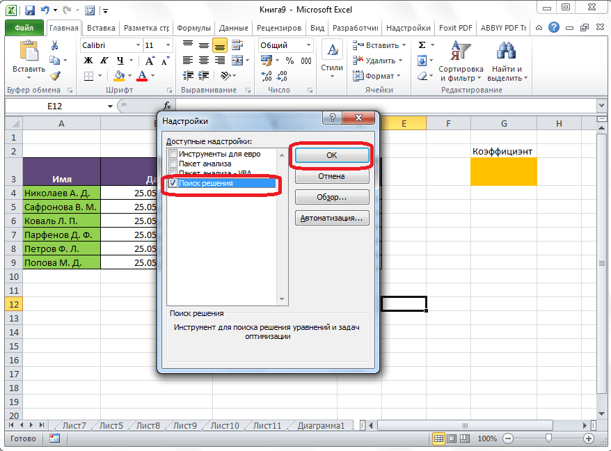
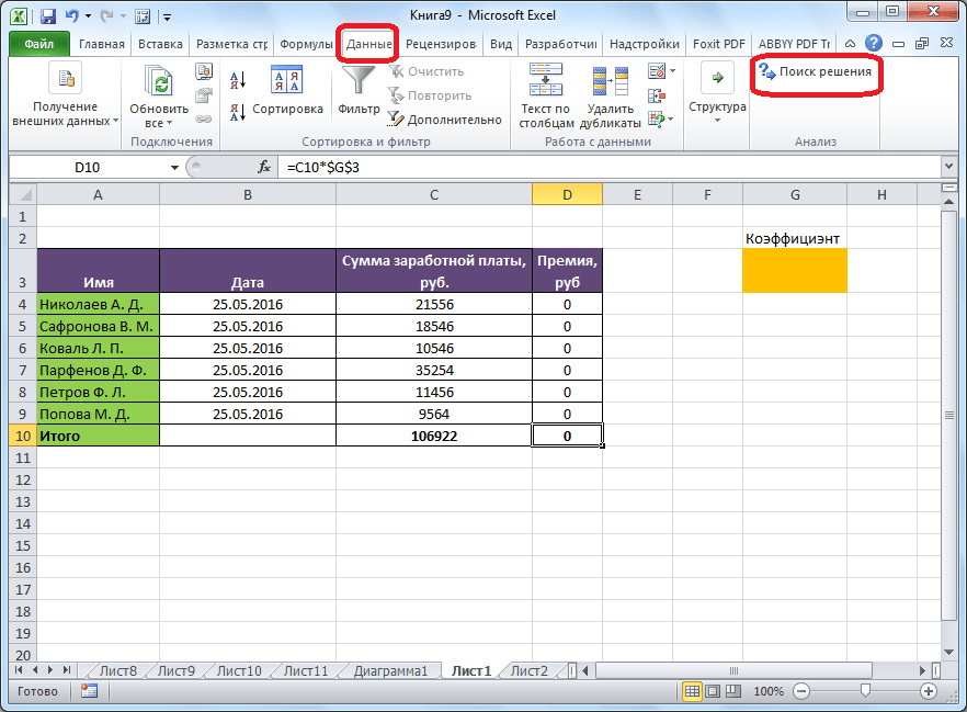
After that, a button to start the Search for solutions function will appear on the Excel ribbon in the Data tab.
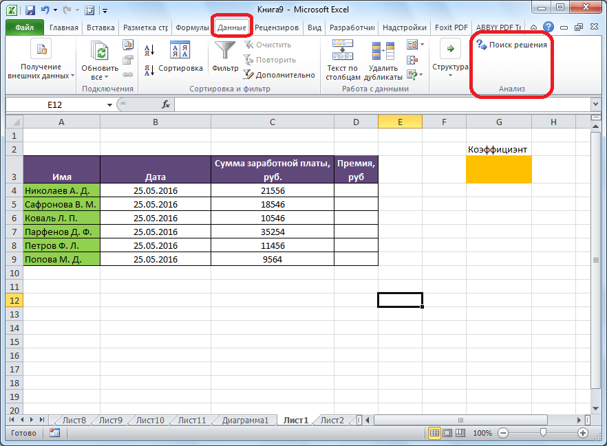
Preparing the table
Now that we have activated the function, let's see how it works. The easiest way to imagine this is with a specific example. So, we have a table of wages of employees of the enterprise. We need to calculate the bonus for each employee, which is the product of the wages indicated in a separate column by a certain coefficient. At the same time, the total amount of funds allocated for the premium is 30,000 rubles. The cell in which this amount is located has the name of the target one, since our goal is to select the data exactly for this number.
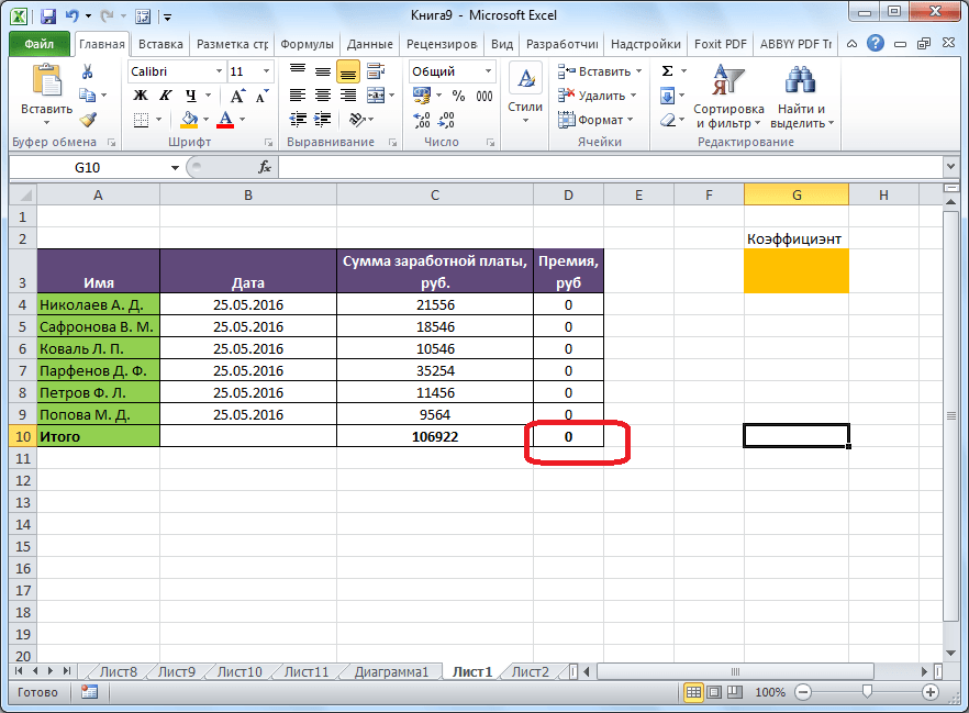
The coefficient that is used to calculate the amount of the premium, we have to calculate using the Search for solutions function. The cell in which it is located is called the desired one.

The target cell and the target cell must be related to each other using a formula. In our particular case, the formula is located in the target cell, and has the following form: "\u003d C10 * $ G $ 3", where $ G $ 3 is the absolute address of the sought cell, and "C10" is the total salary from which the bonus is calculated employees of the enterprise.

Launching the Find Solution Tool
After the table is prepared, being in the "Data" tab, click on the "Search for a solution" button, which is located on the ribbon in the "Analysis" toolbox.
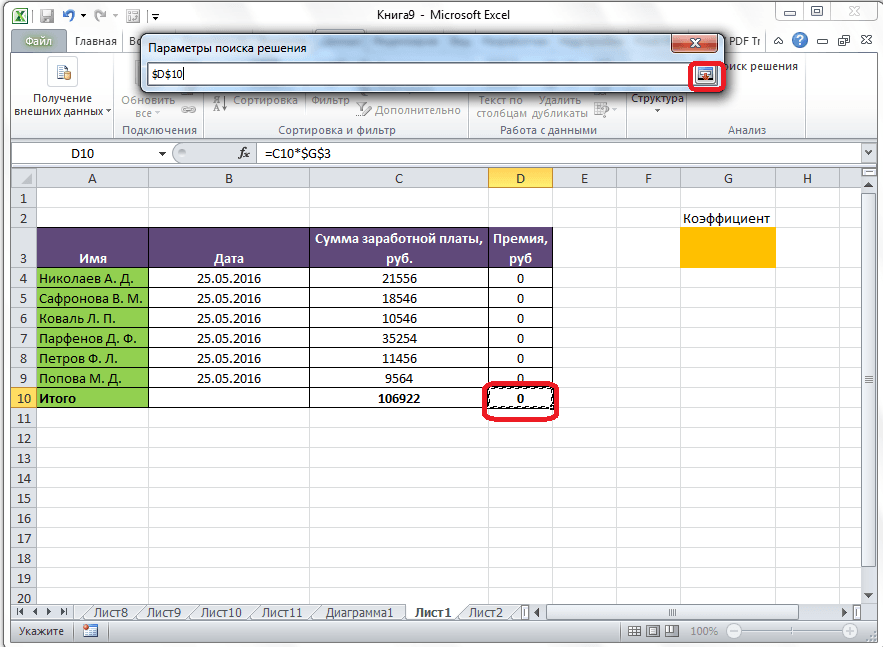
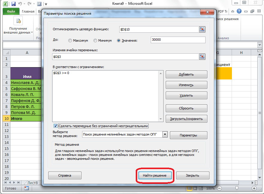
The parameters window opens, in which you need to enter the data. In the field "Optimize the objective function" you need to enter the address of the target cell, where the total bonus amount for all employees will be located. This can be done either by typing the coordinates manually, or by clicking on the button located to the left of the data entry field.
![]()
After that, the parameters window will be minimized, and you can select the desired cell of the table. Then, you need to click on the same button again to the left of the form with the entered data to expand the parameters window again.
Under the window with the address of the target cell, you need to set the parameters of the values \u200b\u200bthat will be in it. It can be a maximum, a minimum, or a specific value. In our case, this will be the last option. Therefore, we put the switch in the “Values” position, and in the field to the left of it we write the number 30,000. As we remember, this number, according to the conditions, is the total amount of the bonus for all employees of the enterprise.
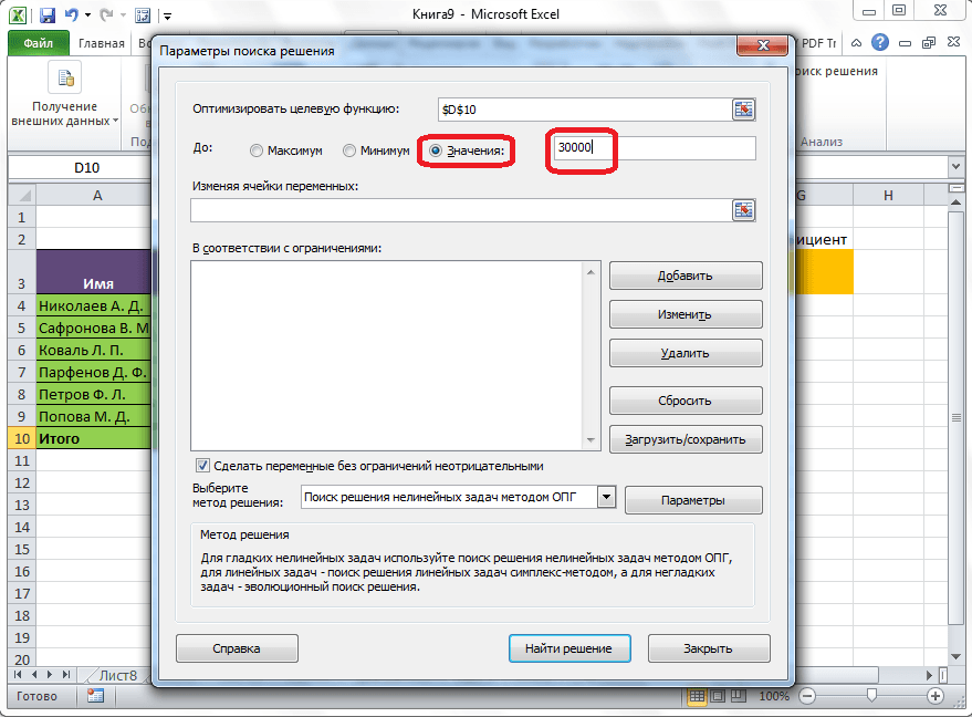
Below is the field "Changing variable cells". Here you need to indicate the address of the desired cell, where, as we remember, the coefficient is located, by multiplying the basic salary by which the amount of the bonus will be calculated. The address can be written in the same ways as we did for the target cell.

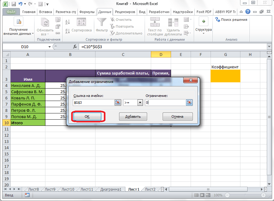
In the "According to restrictions" field, you can set certain restrictions for the data, for example, make the values \u200b\u200bwhole or non-negative. To do this, click on the "Add" button.

After that, the window for adding a constraint opens. In the "Link to cells" field, write the address of the cells with respect to which the restriction is introduced. In our case, this is the desired cell with a coefficient. Then we put down the required sign: “less than or equal”, “greater than or equal”, “equal”, “integer”, “binary”, etc. In our case, we will choose a greater than or equal sign to make the coefficient a positive number. Accordingly, in the "Restriction" field, indicate the number 0. If we want to configure another restriction, then click on the "Add" button. Otherwise, click on the "OK" button to save the entered restrictions.
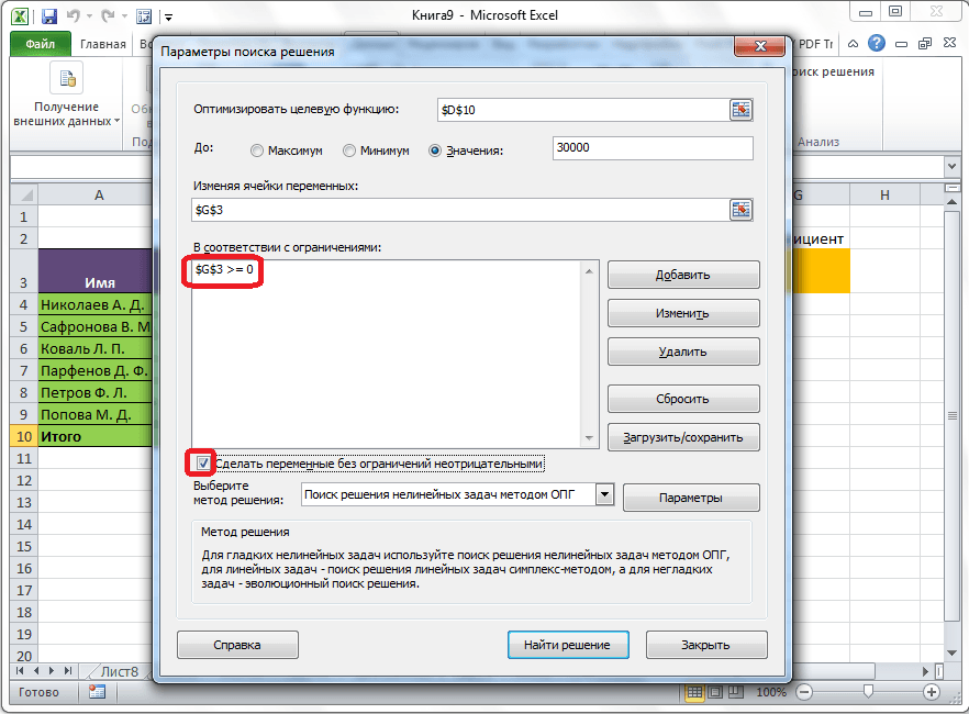
As you can see, after that, the restriction appears in the corresponding field of the solution search parameters window. Also, you can make variables non-negative by checking the box next to the corresponding parameter just below. It is advisable that the parameter set here does not contradict those that you prescribed in the restrictions, otherwise a conflict may arise.
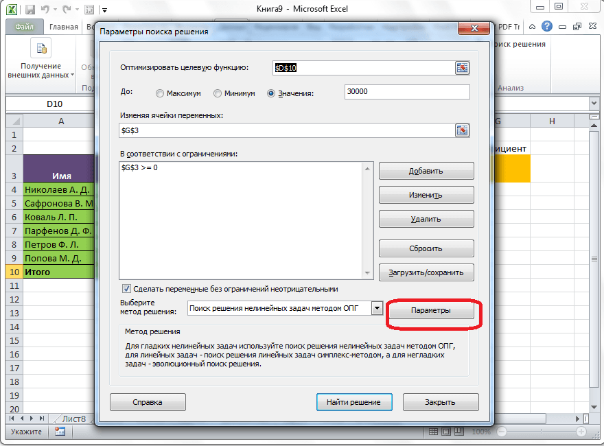
Additional settings can be set by clicking on the "Parameters" button.
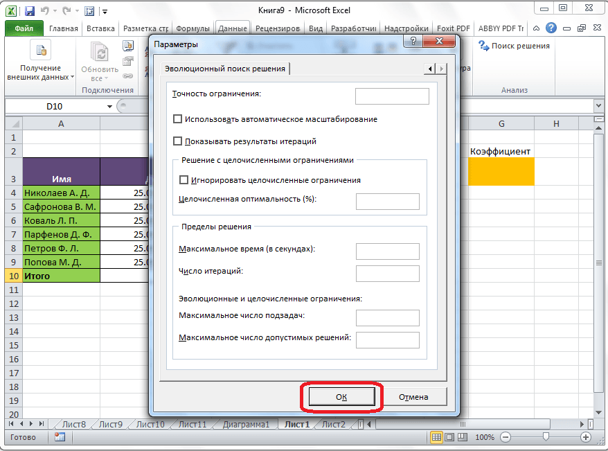
Here you can set the precision of the constraint and the limits of the solution. When the required data is entered, click on the "OK" button. But, for our case, there is no need to change these parameters.
After all the settings are set, click on the "Find a solution" button.
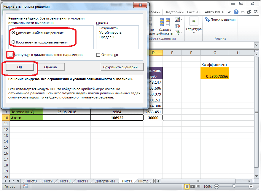
Further, the Excel program in the cells performs the necessary calculations. Simultaneously with the output of the results, a window opens in which you can either save the found solution, or restore the original values \u200b\u200bby moving the switch to the appropriate position. Regardless of the selected option, by checking the box "Return to the options dialog box", you can again go to the search solution settings. After the checkboxes and switches are set, click on the "OK" button.
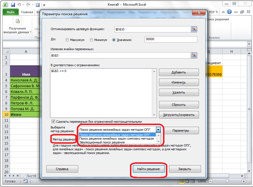
If, for any reason, the results of the search for solutions do not satisfy you, or the program gives an error when calculating them, then, in this case, we return, as described above, to the parameters dialog box. We are reviewing all the entered data, as there may have been a mistake somewhere. If the error was not found, then go to the "Select a solution method" parameter. Here you can choose one of three calculation methods: "Search for a solution to nonlinear problems by the OPG method", "Search for a solution to linear problems by the simplex method", and "Evolutionary search for a solution". By default, the first method is used. We are trying to solve the problem by choosing any other method. If unsuccessful, try again using the last method. The algorithm of actions is the same as described above.
As you can see, the Find a solution function is a rather interesting tool that, if used correctly, can significantly save the user's time on various calculations. Unfortunately, not every user is aware of its existence, let alone be able to correctly work with this add-on. In some ways, this tool resembles the function , but at the same time, it has significant differences with it.
If in excel cell a formula is introduced containing a link to the same cell (maybe not directly, but indirectly - through a chain of other links), then they say that there is a cyclic reference (cycle). In practice, cyclic references are used when it comes to implementing an iterative process, calculating by recurrence relations. In the usual excel mode detects a cycle and issues a message about the situation that has arisen, demanding its elimination. Excel cannot perform calculations because circular references generate an infinite number of calculations. There are two ways out of this situation: eliminate circular references, or allow calculations using formulas with circular references (in the latter case, the number of cycle repetitions must be finite).
Consider the problem of finding the root of an equation using Newton's method using cyclic references. Take a quadratic equation as an example: x 2 - 5x + 6 \u003d 0, a graphical representation of which is shown in. You can find the root of this (and any other) equation using just one Excel cell.
To enable cyclic computing in tools menu / Options / Calculations tab turn on the checkbox Iteration, if necessary, change the number of loop repetitions in the field Limit number of iterations and the accuracy of calculations in the field Relative error (by default their values \u200b\u200bare 100 and 0.0001, respectively). In addition to these settings, we select the option of calculating: automatically or manually... When automatic calculation Excel immediately gives the final result, when calculating manually, you can observe the result of each iteration.
| Figure: 8. Function graph |
Let's select an arbitrary cell, give it a new name, say - X, and introduce into it a recurrent formula specifying calculations by Newton's method:
 ,
,
where F and F1 set, respectively, expressions for calculating the values \u200b\u200bof the function and its derivative. For our quadratic equation, after entering the formula, the value will appear in the cell 2
corresponding to one of the roots of the equation (). In our case, the initial approximation was not specified, the iterative computational process began with the default value stored in the cell X and equal to zero. How do you get the second root? This can usually be done by changing the initial guess. You can solve the problem of specifying initial settings in each case in different ways. We will demonstrate one technique based on the use of the IF function. In order to increase the clarity of the calculations, meaningful names () were assigned to the cells. 
2.2. Parameter selection
When you know the desired result of the formula, but you do not know the values \u200b\u200brequired to obtain this result, you can use the tool Parameter selectionby choosing the command Parameter selection on the menu Service... When you select an option, Excel changes the value in one specific cell until the formula that references that cell yields the desired result.
Take as an example the same quadratic equation x 2 -5x + 6 \u003d 0... To find the roots of the equation, do the following:
Excel uses an iterative (round-robin) process to select the parameter. The number of iterations and precision are set in the menu Tools / Options / Calculations tab... If Excel is performing a complex parameter selection task, you can click Pause in the dialog box Parameter selection result and interrupt the calculation, and then press the button Stepto iterate again and see the result. When solving a problem in step-by-step mode, a button appears Proceed - to return to the normal parameter selection mode.
Let's go back to the example. Again the question arises: how to get the second root? As in the previous case, it is necessary to set an initial approximation. It can be done like this ():
 |
| and |
 |
| b |
| Figure: 11. Finding the second root |
However, all this can be done in a somewhat simpler way. To find the second root, it is enough to put the constant in cell C2 as an initial approximation () 5 and after that start the process Parameter selection.
2.3. Finding a solution
Team Parameter selection is convenient for solving problems of finding a specific target value, depending on one unknown parameter. For more complex tasks, use the command Finding a solution (Solver), which is accessed via the menu item Service / Solution Search.
Tasks that can be solved with Find a solution, in the general setting are formulated as follows:
To find:
x 1, x 2, ..., x n
such that:
F (x 1, x 2, ..., x n)\u003e (Max; Min; \u003d Value)
with restrictions:
G (x 1, x 2, ..., x n)\u003e (Ј Value; i Value; \u003d Value)
Variables sought - worker cells excel worksheet - are called adjustable cells. Objective function F (x 1, x 2, ..., x n)sometimes referred to simply as a goal, must be specified as a formula in a cell in a worksheet. This formula can contain user-defined functions and must depend on (reference) the adjustable cells. At the moment of setting the problem, it is determined what to do with the objective function. You can choose one of the options:
- find the maximum of the objective function F (x 1, x 2, ..., x n);
- find the minimum of the objective function F (x 1, x 2, ..., x n);
- achieve that the objective function F (x 1, x 2, ..., x n) had a fixed value: F (x 1, x 2, ..., x n) \u003d a.
Functions G (x 1, x 2, ..., x n) are called constraints. They can be specified both in the form of equalities and inequalities. Additional restrictions can be imposed on the regulated cells: nonnegativity and / or integer, then the sought solution is sought in the range of positive and / or integers.
This formulation covers the widest range of optimization problems, including the solution of various equations and systems of equations, linear and nonlinear programming problems. Such problems are usually easier to formulate than to solve. And then, to solve a specific optimization problem, a specially designed method is required. Solver has in its arsenal powerful tools for solving such problems: the generalized gradient method, the simplex method, the branch and bound method.
Above, to find the roots of a quadratic equation, Newton's method was applied (section 1.4) using cyclic references () and the tool Parameter selection (). Let's see how to use Finding a solution using the example of the same quadratic equation.
After opening a dialogue Finding a solution () you need to do the following:- in field Set target cell enter the address of the cell containing the formula for calculating the values \u200b\u200bof the optimized function, in our example, the target cell is C4, and the formula in it is: \u003d C3 ^ 2 - 5 * C3 + 6;
- to maximize the target cell value, set the radio button maximum value to position 8, the switch is used to minimize minimum value, in our case, set the switch to the value position and enter the value 0 ;
- in field Changing cells enter the addresses of the cells to be changed, i.e. arguments of the objective function (C3), separating them with the ";" (or by clicking with the mouse while the key is pressed Сtrl on the corresponding cells), to automatically search for all cells influencing the solution, use the button Guess;
- in field Limitations using the button Add to enter all the restrictions that the search result must meet: for our example, you do not need to set restrictions;
- to start the process of finding a solution, press the button Execute.
To save the obtained solution, you must use the switch Save found solution in the opened dialog window Solution search results... After that, the worksheet will take the form shown in. The resulting solution depends on the choice of the initial approximation, which is specified in cell C4 (function argument). If, as an initial approximation in cell C4, enter a value equal to 1,0 , then using Find a solution find the second root equal to 2,0 .
Options governing work Find a solutionset in the window Parameters (the window appears if you click on the button Parameters window Finding a solution), the following ():
- Maximum time - limits the time allotted for the process of finding a solution (the default is 100 seconds, which is enough for problems with about 10 restrictions, if the problem is of large dimension, then the time must be increased).
- Limit number of iterations - another way to limit the search time by setting the maximum number of iterations. The default is 100, and, most often, if the solution is not obtained in 100 iterations, then with an increase in their number (in the field you can enter a time not exceeding 32767 seconds) the probability of getting a result is small. Better to try to change the initial guess and start the search process again.
- Relative error - specifies the precision with which the cell matches the target value or the approximation to the specified limits (decimal fraction from 0 to 1).
- Tolerance - set in% only for tasks with integer constraints. Finding a solution in such problems, it first finds the optimal non-integer solution, and then tries to find the nearest integer point, the solution at which would differ from the optimal one by no more than the number of percent indicated by this parameter.
- Convergence - when the relative change in the value in the target cell over the last five iterations becomes less than the number (fraction from the interval from 0 to 1) specified in this parameter, the search stops.
- Linear model - this checkbox should be enabled when the objective function and constraints are linear functions. This speeds up the process of finding a solution.
- Non-negative values - this flag can be used to set constraints on variables, which will allow you to search for solutions in the positive range of values \u200b\u200bwithout specifying special constraints on their lower bound.
- Automatic scaling - this flag should be enabled when the scale of the values \u200b\u200bof the input variables and the objective function and constraints differ, possibly by orders of magnitude. For example, variables are set in pieces, and the objective function that determines the maximum profit is measured in billions of rubles.
- Show iteration results - this checkbox allows you to enable a step-by-step search process, showing the results of each iteration on the screen.
- Estimates - this group serves to indicate the method of extrapolation - linear or quadratic - used to obtain the initial estimates of the values \u200b\u200bof variables in each one-dimensional search. Linear serves to use linear extrapolation along the tangent vector. Quadratic serves to use quadratic extrapolation, which gives better results when solving nonlinear problems.
- Differences (derivatives) - this group serves to indicate the method of numerical differentiation, which is used to calculate the partial derivatives of target and limiting functions. Parameter Direct it is used in most tasks where the rate of change of restrictions is relatively low. Parameter Central used for functions with a discontinuous derivative. This method requires more computations, but its application can be justified if a message is displayed that it is not possible to obtain a more accurate solution.
- Search method - serves to select an optimization algorithm. Newton's method was discussed earlier. IN Conjugate gradient method less memory is requested, but more iterations are performed than Newton's method. This method should be used if the task is large enough and it is necessary to save memory, and also if the iterations give too little difference in successive approximations.
- when saving an Excel workbook after finding a solution, all values \u200b\u200bentered in dialog boxes Finding a solutionare saved along with the worksheet data. One set of parameter values \u200b\u200bcan be saved with each worksheet in the workbook Find a solution;
- if within one Excel worksheet it is necessary to consider several optimization models (for example, find the maximum and minimum of one function, or the maximum values \u200b\u200bof several functions), then it is more convenient to save these models using the button Options / Save Model window Finding a solution... The range for the saved model contains information about the target cell, about the changed cells, about each of the constraints and all the values \u200b\u200bof the dialog Parameters... The choice of a model for solving a specific optimization problem is carried out using the button Parameters / Load model dialogue Finding a solution;
- another way to save search parameters is to save them as named scripts. To do this, click on the button Save script dialog box Search results for solutions.
In addition to inserting optimal values \u200b\u200binto the cells being changed Finding a solution allows you to present the results in the form of three reports: results, Sustainability and The limits... To generate one or several reports, you must select their names in the dialog window Solution search results... Let's consider each of them in more detail.
 |
| Figure: 15. Sustainability report |
The Limits report contains information about the limits within which the values \u200b\u200bof the modified cells can be increased or decreased without violating the task constraints. For each cell that you change, this report contains the optimal value as well as the smallest values \u200b\u200bthat the cell can accept without violating the constraints.