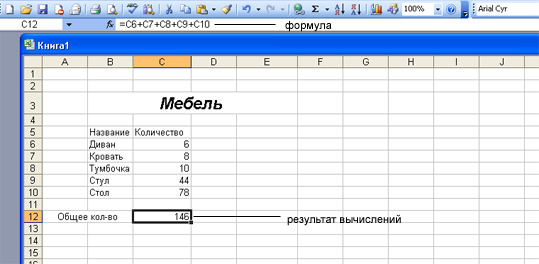
Create spreadsheet in excel
Create spreadsheets microsoft program Excel
Computer science, cybernetics and programming
On the screen, the cells of the table sheet are separated by grid lines. The right part is used to display the contents of the current cell. To switch to edit mode for cell content in the formula bar, press F2 or click on the right side of the formula bar. A button in the formula bar serves to confirm data entry or change the contents of a cell and corresponds to the action of the Enter key.
Laboratory work No. 7
7 Creation of spreadsheets by the program Microsoft Excel
7.1 Purpose of work.
The purpose of this laboratory work is to get acquainted with some of the main features of the Russian version of the spreadsheet programMicrosoft Excel (version 7.0) designed to run on a computer running operating systems of the familyWindows, obtaining skills in drawing up and designing a spreadsheet, presenting data using diagrams.
7.2. Microsoft Excel program
7.2.1 Purpose and capabilities
Microsoft Excel 7.0 is an application from the Microsoft Office package. The basis of the program is a computational module, with the help of which data (textual or numerical) is processed in tables. To create presentation graphics, a module of diagrams is used, which allows obtaining diagrams of various types on the basis of numerical values \u200b\u200bprocessed using a computing module. Using the database module inExcel access to external databases is implemented. The programming module allows the user not only to automate the solution of the most complex problems, but also to create his own program shell. In the seventh versionExcel you can create macros using a programming language dialectVisual Basic for Applications.
Excel can be used both for solving simple accounting problems, and for drawing up various forms, business graphics and even a full balance sheet of the company. With powerful math and engineering functions usingExcel you can also solve many problems in the field of natural and technical sciences.
Excel has great potential and is undoubtedly one of the best programs their class. However, its study and application is useful not only for this reason. Its prevalence plays an important role. This program is installed on almost any computer. Ability to useExcel is very important.
Possibilities of using the programExcel go far beyond those that will be considered in the course of this work. You are invited to familiarize yourself with the possibilities of working with tables, charts, list data.
Maximized program windowExcel 7.0
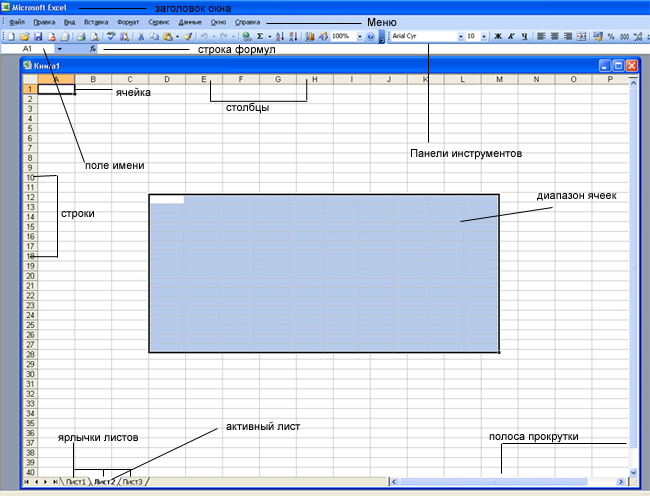
After starting Excel the expanded program window will be displayed on the monitor screen. It is shown in Figure 65.
Screen structure when working withExcel a lot like the screen layout of other appsMicrosoft office.
A document created in Excel is called a workbook (book ). The book includes sheets of spreadsheets, which are called worksheets (worksheet ) or just sheets of tables.
A new workbook usually contains three blank sheets of tables. Sheets of tables have the standard names Sheet 1, Sheet 2, Sheet 3, etc. The number of sheets and their name can be changed.
The entire space of each sheet of the spreadsheet is broken up into 1,048,576 rows and 16,384 columns. On the screen, the cells of the table sheet are separated by grid lines. Rows are denoted by numbers from 1 to 1048576, columns are denoted by Latin letters from A to XFD.
Thus, the following structure is obtained: a book, which is a separate file, consists of sheets, and each sheet consists of cells. The first cell has the address A1, and the last XFD1048576
Figure 65 - Expanded program windowExcel
The maximized Excel window (Figure 65) is similar to the maximized windows of Microsoft Office 2007. This program uses a new ribbon interface.
The ribbon, as in other programs, has a set of tabs. Each tab contains a group or groups of tools. In a programmeExcel the following tabs are available:
the main - this tab is available by default at startupExcel ... It contains the main tools designed to perform basic operations for editing and formatting (formatting) text in cells, formatting the cells themselves, manipulating cells, etc. (see figure 66).
Figure 66 - the "The main"
Insert - designed to be inserted into spreadsheet all kinds of elements: pictures, clips, inscriptions, headers and footers, all kinds of graphs and diagrams (see Figure 67).
Figure 67 - the "Insert"
Page layout - contains tools focused on setting and configuring various parameters of page layout, margins, colors and page orientation, indents, etc. (see figure 68).
Figure 68 - the "Page layout"
Formulas - this tab for the convenience of setting and using formulas in the cells of the spreadsheet. The function wizard, the function library, and the reference value window are accessible from this tab. (see figure 69).
Figure 69 - the "Formulas "
Data - the tools of this tab are focused on operations with data contained in table cells: sorting, applying a filter, grouping, etc. In addition, the tab contains tools that allow you to transfer data from other applications to the table (see Figure 70).
Figure 70 - the "Data"
Peer review - contains such tools as inserting and editing notes, protecting a spreadsheet or individual sheets, etc. (see figure 71).
Figure 71 - the "Reviewing "
View - the tab is intended for setting the mode of viewing documents in the program window (see Figure 72).
Figure 72 - the "View"
Just like on the tapeWord 2007, on the Excel ribbon 2007 all tools on the tabs are combined into groups, access to additional group tools is the same as inWord 2007 defined by pressing a button... Similar to Word 2007 buttons in Excel 2007 can be simple and two-part. PackageExcel 2007 has a "Quick Access Toolbar" that is highly customizable. Setting is carried out in the same way as the programMicrosoft Word 2007.
pay attention toformula bar , which is designed to process the contents of table cells. This line is divided into three parts. The right part is used to display the contents of the current cell. Data editing can be done directly in the cell itself or in the formula bar. To switch to the mode of editing the contents of a cell in the formula bar, press the key
Button that is on the formula bar is used to undo the last action. Button in the formula bar serves to confirm data entry or change the contents of a cell and corresponds to the action by
7.2.3. Mouse pointer in Excel 7.0
As you move within the Excel 7.0 window, the appearance of the mouse cursor changes.
In normal mode, the mouse pointer looks like an arrow. With it, you can select various elements of the window, activate them by double-clicking or perform a drag-and-drop operation.
Being inside the worksheet, the mouse cursor looks like a cross. In this case, after clicking, the cell on which the cursor is positioned becomes active.
When placed over a fill handle in the lower-right corner of a cell, the mouse pointer appears as a black cross. Thus, the program informs about the possibility of using the function "autocomplete ". This function allows the user to represent frequently occurring sequences of values \u200b\u200b(for example, namesmonths) as a list. If a cell contains a list item, then the remaining items of the same list can be added to the worksheet automatically using the function "Autocomplete".
Autocomplete cursor "Can also be used when copying formulas.
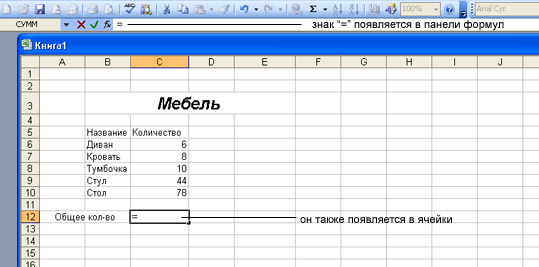
Formulas are expressions that are used for calculations on a page. The formula begins with an equal sign (\u003d). The formula contains operators. An operator is a sign or symbol that specifies the type of evaluation in an expression. There are mathematical, logical, comparison and reference operators. Operators for calculations use constants, i.e. constant values \u200b\u200bover which calculations are performed, and references to cells containing data for calculations.
A formula can also contain items such as functions.Function Is a standard formula that returns the result of performing certain actions on values \u200b\u200bthat act as arguments. Functions allow you to simplify formulas in worksheet cells, especially if they are long or complex.
Cell references used in formulas and functions can beabsolute and relative... An absolute cell reference when copying a formula with the autocomplete cursor selects the value for calculations only from the cell indicated by that reference. No forwarding to other cells occurs. An absolute reference is indicated by the $ sign in the row and column names of the reference. For example $A $ 7, a link to the contents of cell A7 and no matter how we copy our formula, there will always be a link to the data in this cell.
In Excel, in addition to absolute cell references, it also usesrelative links. When creating a formula, these references usually take into account the location relative to the cell containing the formula. The link can be entirely relative column-relative and row-relative (e.g. C1). Or by a mixed reference relative column and absolute row (C $ 1), absolute column and relative row ($ C1). Links in which only a column or only a row is fixed are called mixed links. You can also change a relative reference in a formula to an absolute reference by pressingF 4.
Thus, a formula is a collection of values, references to other cells, named objects, functions and operators, allowing you to get a new value.
If the cursor becomes an input cursor, the user is able to enter or edit data. When the window is resized, the cursor becomes a multidirectional arrow. A multidirectional arrow, crossed out by a line, appears on the screen if the cursor is between two elements whose borders can be changed (for example, between the headings of rows or columns). The cursor, which looks like two parallel lines with arrows, is used to divide the worksheet into several subwindows (panels) using split markers. After pressing the key combination
7.2.4. Building a table
Building a table in Excel 7.0 is done in a worksheet. The worksheet is divided into rows and columns, with the intersections of rows and columns forming cells. In each cell, the user can enter certain data. The cell into which data will be entered must first be activated. Activation is carried out by clicking on a cell or by moving the cell pointer using the cursor keys.
A cell of a spreadsheet can contain information of various types: text, numeric values, and formulas. In addition, each cell can be formatted separately without being affected by the formatting options. When typing excel data automatically recognizes their type.
As soon as at least one character is entered in a cell, the contents of the cell are immediately displayed in the formula bar. At the same time, this line will display the image of three buttons that are used to process the contents of the cell.
After confirming that a numeric value has been entered into a cell, it will be automatically right-aligned; the program will automatically left-align the text data. You can set a different alignment parameter for this cell. When specifying an alignment, for example, to the left, the entered new numeric values \u200b\u200bwill be aligned to the left.
If the length of the text entered into a cell exceeds the current value of the width of this cell, then after completing the input, the text will either be fully represented in the table, covering the empty cells that are located on the right, or will be truncated along the right edge of the cell if the adjacent cell contains some or information. All text will be fully represented in the formula bar when you move the cell pointer to a cell with this text. In addition, if a cell is enteredtext , which was already entered into the adjacent cell, then the auto-substitution function is triggered.
If, due to the insufficient width of the cell, the numerical values \u200b\u200bin it cannot be fully represented, then the screen will display the corresponding number of sharp “#” symbols, while the contents of the cell will be fully represented in the formula bar.
If a cell is entered formula , then immediately after the input is completed, calculations are performed, and the result of the calculations is displayed in the cell. Formulas in Excel must begin with a mathematical operator. For example, after you enter the formula \u003d 1 + 6, the number 7 appears in the cell, but the formula appears in the formula bar as the actual content of the cell. If you enter 1 + 6, then this value will be interpreted by the program as text. A formula can also begin with plus (+) or minus (-) signs. These signs refer to the first numeric value in the formula.
After setting the formula in the cell, a message may appear about error. For example, if you enter the value=1/0 , then it will be interpreted by the program as a formula, and Excel will immediately try to calculate. However, after a while, a message will appear in the cell\u003d DIV / 0! , by which it will not be difficult to determine the nature of the error.
Through selection of cells data entry can be somewhat simplified. To select a range of cells, move the mouse pointer with the left button pressed in the required direction. If you want to perform this operation using the keyboard, you should place the cell pointer in its original position, press the key
One of the cases where selection of a range of cells is used is when using the autocomplete function of cells. For example, if you need to fill several columns with the same values \u200b\u200b(see figure 73):
|
The cost of computers (inU SD) |
|||
|
1050 |
1050 |
||
|
Computer for gamesCore i 7 870 |
1570 |
1570 |
|
|
1400 |
1400 |
||
Figure 73 - An example of data entry into a table
(In Figure 73, note the columnsC and D).
In order to fill the range of cells C13 - D15, you need to do the following:
- Enter in cells С13, С14 and С15, respectively, the values: 330; 560; 850.
- Activate cell C13 by clicking on it.
- While holding down the left mouse button, move the cursor down to cell C15, thus selecting the range of cells C13-C15.
- Position the mouse pointer over the fill handle of the selected range of cells (in the lower right corner of the range). Keeping the left button pressed, move the fill handle to column D and release the mouse button. Thus, the cells of the range D13 - D15 will be automatically filled.
To select an entire column , you must click on its title.Line stands out similarly. When selecting a column using the keyboard, place the cell pointer in the selected column, and then press the key combination
If incorrect data was entered into a cell, its contents must beedit... The fastest and in a simple way Changing the contents of a cell is overwriting the old new information, while the previous contents of the cell are automatically deleted. In case of minor errors, it is better not to rewrite, but to edit the data in the cells. To do this, activate the edit mode by double-clicking on the cell, after which a blinking input cursor will be presented to the right of the cell content. You can enable editing mode using the keyboard by placing the pointer on the desired cell and pressing the key
In edit mode, the contents of the cell will be presented in the table in full, regardless of whether the adjacent cell is filled or not. Cell content can be edited both in the table itself and in the formula bar.
IN Excel content a separate cell may bemoved or copied ... The contents of the cells to which the transfer is carried out are automatically deleted. To avoid this, you must insert blank cells in the area of \u200b\u200bthe spreadsheet where you want to transfer data.
The difference between the move operation and copy operation is that when moving, the contents of the cells in the original position are deleted. When copying, the contents of the cells are preserved in their original position. To move a range of cells using the manipulator, you must select the desired cells (this applies only to adjacent cells). Then you should place the mouse cursor anywhere on the border of the selected range and drag, holding down the left mouse button, the entire range to a new position. When the manipulator button is released, the contents of the selected cells are removed from their original position and inserted into the current position. If you hold down the key while performing this operation
7.2.5. Table decoration
Excel provides many different features that allow you to design your tables in a professional manner. By varying different kinds font, line thickness and location, background color, etc., you can achieve the most visual representation of information in the table.
Before executing any command in Excel, you should select a cell (range of cells), which will be affected by the command. This is also true for commands for setting formatting parameters in a table. If a range of cells is not selected, then formatting options are set for the active cell.
To display numerical values Excel uses the General number format by default, and values \u200b\u200bare presented in the table as they were entered on the keyboard. When you enter numeric information, the cell contents are assigned one of the numeric formats supported by Excel. If the format is “unfamiliar”, then the entered numerical value is interpreted by the program as text (for example, 5 coupons). To assign a number format to a cell or group of cells, you can use the commandCells of the Format menu using the Format command context menu cells or keyboard shortcut
- general;
- numerical;
- monetary;
- financial;
- the date;
- time;
- percentage;
- fractional;
- exponential;
- text;
- additional;
- (all formats).
After selecting a specific category, the formats contained in it will be presented in the list box on the right. To set the format of cells, select its name from the list field. Note that in some cases, after setting the format, more space will be required to represent the contents of the cells.
When choosing monetary format numerical values \u200b\u200busually cannot be represented in the table due to insufficient width of the cells. In this case, the contents of the cell are displayed using the special characters hash “#”. Only after a corresponding increase in the width of the column will the data in the cells be presented in normal form again.
In Excel, there is another, more convenient way to format cells: using the buttons on the toolbar. For example, a currency format can be assigned to cells using the button.
Change column width the worksheet is best done with the mouse. You need to move the mouse cursor to the column header area. When the cursor is positioned exactly between two column headings, the cursor becomes a black double-headed arrow. In this mode, you can move (while holding down the left button) the right edge of the left column. After you release the left mouse button, the new column width will be fixed. Double-clicking in this mode sets the column to the optimal width. By choosing the command "AutoFit Column Width "From the" Format "list on the" Home "tab, you can instruct the program to determine the optimal column width. The width is set depending on the length of the contents of the cells. This will set its own optimal width for each column. Height of lines set depending on the type of font used. Changing the row height is done in the same way as changing the column width. You can set the row height (and the column width, respectively) in the dialog box Line height , which opens with the command "Row Height ”in the Format list on the Home tab.
When you enter data in Excel, the contents of the cells are automatically aligned. But the alignment for a cell can be set: using the buttons of the Alignment group on the Home ribbon and in the Format Cells dialog box on the Alignment tab.
Adding frames, colors, palettes, and shadows to make it easier for other users to work with the data contained in the worksheet can be achieved more clearly. You can set the parameters you need using the buttons in the group «Font ", on the" Home "tab or in the dialog box "Cell format ".
If you don't want to waste time formatting your table manually, you can use styles in Excel. You can also use the function "Autoformat " ... To do this, it is convenient to get the button on the quick panel - "AutoFormat". Auto Format function works as follows: Microsoft Excel parses the range of contiguous cells pointed to by the cursor and automatically applies a format based on the position of headings, formulas, and data.
7.2.6. Calculations in MS Excel
Excel program is designed to perform calculations involving the presentation of data in tabular form. Therefore, the Excel worksheet looks like a table.
Each cell in the worksheet can contain text or a numeric value that can be used in calculations. The cell can also contain a formula. In this case, the result presented in the cell depends only on the contents of those cells that are referenced in this formula.
A formula can contain functions and mathematical operators, the order of which is the same as in mathematics. The result of evaluating formulas that include arithmetic operators are numeric values, and in the case of comparison operators, logical values \u200b\u200b"True "or" False " ... Table 1 presents arithmetic operators in descending order of their precedence in calculations.
For example, to get the total number of computers sold in July in cell B9, you should activate this cell, enter an equal sign, and then sequentially the addresses of all cells from B5 to B8, connecting them with the addition operator. As a result, the formula entered into cell B9 will look like this:
B5 + B6 + B7 + B8
Table 1
Arithmetic operators
|
Operator |
Value |
|
Open parenthesis |
|
|
Close parenthesis |
|
|
Multiply |
|
|
Split |
|
|
To fold |
|
|
Subtract |
|
|
Equally |
|
|
Less |
|
|
Less or equal |
|
|
More |
|
|
More or equal |
|
|
Not equal |
When you finish entering the formula, press
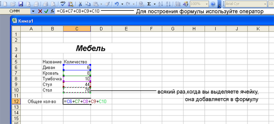
You can use various techniques to define the formula. In the example above, the formula was entered using keyboard input. However, there is another way: after entering the equal sign, you must click on the cell that should be indicated in the link first (B5). This cell will be framed with a dashed creeping box, and its address will appear in the final cell. Next, you enter the addition operator, and then click on the next cell, and so on.
You can also use numerical values \u200b\u200bin formulas directly by connecting them using mathematical operators. A combination of cell addresses and numeric values \u200b\u200bis also possible.
You can also use the button to calculate amounts (for example, the total number of computers sold in July)., which is located on the tape "Formula ".
Once you select a range of cells, you can get information about it by looking atstatus linelocated at the bottom of the main Excel window. If the status bar is configured accordingly, you can see the number of numbers selected in the range, their sum, average value, minimum and maximum.
Call the context menu of the status bar and in the menu that opens, specify what kind of information you want to receive on the status bar.
In Excel for multiple cells that make up an array interval one general formula can be given - array formula... In our example, taxes are 30% of gross revenue. You can enter the formula in cell B21:\u003d B20 * 0.30, and then copy to the rest of the cells. But you can use an array formula. To do this, select cells B21 - D21, which will be the array interval, and enter the formula in cell B21:\u003d B20: D20 * 0.30. In order for the effect of the entered formula to apply to the entire array, you should complete its input by pressing the key combination
In calculations, a wide variety of formulas can be used, serving, for example, to determine the sine, tangent, average value. Excel provides the user with many special functionsin which these formulas are already embedded. Specifying the values \u200b\u200bto which this or that function should be applied,happens by specifying arguments. The way of defining functions is always the same, the only difference is in the number of arguments that must be specified when defining a function:\u003d FUNCTION NAME (Arguments)
For example, a company's net income is defined as the difference between gross revenues and the amount of taxes and costs. In cell B23 you should enter:\u003d B20-SUM (B21; B22). SUM function name unambiguously indicates the nature of the operation performed with its help.
Sometimes the function itself serves as an argument to another function. These functions are called nested functions.
Functions are best handled withFunction Wizards - in this case, the required arguments are specified in the dialog box, since it is possible to make a mistake when entering a function from the keyboard. For example, if the user forgets to provide a required argument when typing on the keyboard, an error message appears on the screen. An error message is also displayed if the number of closing parentheses does not match the number of opening ones (for example, when specifying nested functions), as well as if other errors were made.
Launch the Function Wizard you can select the command "Function "on the Formula ribbon "Or by activating the key combination
Formulas tab »On the tape of the packageMicrosoft Excel 2007 is shown in Figure 69.
To simplify the work with the programFunction wizard individual functions are grouped thematically. You can set arguments different ways... For example, as arguments to the functionAVERAGE (calculating the average) from one to 30 values \u200b\u200bcan be specified. There is a separate input field for each argument in the dialog box. The input cursor is in the input field of the first argument. In this input field, as the Number 1 argument, you can specify a numeric value (for example, 30 or 45), a cell address (C4), or a cell range address. After specifying the first argument in the Value field in the upper right corner of the dialog box, the result of executing the function with existing arguments will be presented. The dialog also displays an input field for the next argument. When you finish entering the arguments, click the "OK" button, and the result of the calculation will be presented in the corresponding cell.
If errors were made when defining the formula, the result of its calculation will be the so-callederror value that appears in the cell. To make it easier to find the error, you can set the display mode in the cells of the formulas instead of the results of calculations performed by these formulas. To do this, get the button on the quick access panel - « Show formulas". The width of the columns will be automatically increased to provide the user with a better view.
Depending on the type of error that occurred, the cell containing the formula is written different meanings... The first character of the error value is a hash "#" followed by text. The error value text can end with an exclamation mark or a question mark. To resolve the error, select the cell containing the error value. The formula bar displays the formula it contains.
Below are some examples of error values \u200b\u200bwith a brief explanation of them. You can not read them now, but refer to these examples in case one of the listed errors occurs during the execution of work. #NUMBER!
In case of violation of the rules of mathematics, the value of the error will be presented in the cell #NUMBER! Typically, this value appears after changing the content in the influencing cell. For example, if as a function argumentROOT (Square root of a number) set a reference to a cell with a positive value, and at the next stage, change the contents of the influencing cell by entering a negative value, then an erroneous value will appear in the final cell#NUMBER! This error value usually appears when using functions. Look in the help subsystem for what requirements function arguments must meet, and check if the values \u200b\u200bin dependent cells meet those requirements.#NAME?
When defining functions, their names can be written in both uppercase and lowercase letters. Lowercase letters in function names will be automatically converted to uppercase if the program recognizes the input value as a function name. For example, if you specify the function name in the formulaMIX instead of MAX , then the error value will appear in the cell#NAME? since the program cannot find the specified name either among the function names or among the range names. Check the spelling of the function name or insert the function with... # N / A. This error value can appear in a cell when using some functions if the argument is a reference to a cell that does not contain data. The user can set the value in the influencing cell # N / A! , which will be presented in the summary cell to indicate that more data must be entered into the table.#VALUE! If an argument of an invalid type was specified, then an error value will appear in the cell # VALUE! If this error occurs, you need to check, using the help subsystem, whether the argument types for this function are valid.
7.2.7. Graphical presentation of data using charts
For creating and formatting charts, Excel provides the user with a large number of different functions that allow, for example, to select one of the many chart types or to format a legend. The legend describes which data is represented in the chart by a certain color.
For example, in a diagram, when completing an assignment for a lab, cost data can be represented yellow, data on the gross revenue of the enterprise in each month (in July, August and September) - in purple, etc.
In this paper, you are invited to use a diagram to present data on gross revenues, taxes, costs and net income of the enterprise (as instructed by the teacher). To do this, follow these steps.
- Select a range of cells containing row and column labels, which will later be used as labels for the X axis. In our example, these are cells A3 - D3.
- While holding down the key
, select the range of cells (A20-D23), according to the values, from which the diagram will be built. Then let go . - On the "Insert" tab select the required type and type of diagram. For example, a histogram.
Working with a diagram, the user gets additional buttons on the "Design", "Layout" and "Format" tabs in the "Working with Diagrams" tab group. These tabs are shown in Figures 73,74,75.
Figure 73 - The "Constructor" tab
Figure 74 - Tab "Layout"
Figure 75 - Tab "Format"
Using the buttons on these tabs, you can change the data for building a chart, its layout and styles, the name of the chart and its axes, etc. If the formatting of the chart elements is specified on the Format tab, then the Layout tab indicates which elements should be present on diagram.
To remove any of the diagram elements, select it and press the button «Del ”on the keyboard.
In addition, on the diagram, you can build the so-calledtrend line ... This line is built on the basis of an existing chart and allows you to visually see the trend in data changes: they increase, decrease, or do not change. To add a trend line, go to the “Layout ", Select the button"Analysis "And in the opened gallery select"Trend line ", and then the line type.
For the convenience of calculations, you can create pop-up notes for cells. Position the cursor over a cell. On the Review tab, select the Insert Note button. Enter the explanatory text in the window that appears. The fact that a cell contains a note will be indicated by a small red triangle in its upper right corner.
7.3 Work order
- Carefully study the guidelines for laboratory work.
- Obtain permission to perform work from a teacher.
- After turning on the computer and booting the system, start Excel, expanding its window to full screen
- Creating a table
4.1. Key in the table heading: "Determination of Net Income of Computer Ltd".
4.2. In the third line, enter the names of the months using the autocomplete cursor:
4.3. Enter the following text data in cells A4 - A11:
|
‘Computer sales data |
|
|
Core i3 540 multimedia computer |
|
|
Computer for gamesCore i 7 870 |
|
|
AMD Phenom II X4 955 Gaming Computer |
|
|
Intel Core 2 Duo T6570 (2.1 GHz, 2 MB, 800 MHz) / Memory: DDR3 3072 MB |
|
|
Total |
|
|
‘Cost of computers (in USD) |
4.4. Copy the range of cells A5 - A8 to cells A12 - A15.
4.5. Enter in cells A17 - A23:
|
USD rate |
|
|
Gross proceeds |
|
|
Tax |
|
|
Expenses |
|
|
Net income |
5 . Entering data into a table
Enter in the cells the missing numerical values \u200b\u200bof prices for computers, as well as data on computer sales (choose prices from the Internet, and guess the number of sales yourself, guided by the situation on the computer market and the size of your company).
6. Determining the total number of computers sold.
Using the buttonand with the autocomplete function, calculate the total number of computers sold in each month (on line 9).
7 . Using formulas.
7.1. Calculation of gross revenue.
Sequentially performing clicks with the left mouse button on the corresponding cells and using the keys<+> and<*>, enter the formula in cell B20:
\u003d (b 5 * b 12+ b 6 * b 13+ b 7 * b 14+ b 8 * b 15) * b 17
Fill in cells C20 and D20 using the auto-complete function.
7.2. Taxes.
Let's say taxes are 30% of gross revenues. Fill in cells B21 - D21 using the array formula
("Taxes" \u003d "Gross Revenue" * 0.30).
Fill in the Cost line with the numerical values \u200b\u200bthat you consider appropriate.
7.3. Net income.
Net income is calculated as the difference between gross revenue and taxes and costs.
8. Table decoration.
Format the range of cells A3-D23 in the format “Plain" using the button "Autoformat ".
Then select cells A12 - A15 and deselect them using the button on the toolbar.
To design a table heading, select a font size of 12 points, bold (use the buttons on the toolbar) and highlight the heading in red or some other color.
To assign a currency style to cells B17-D23, use the "Monetary format "and then optimize the column widths.
Remove the table grid from the worksheet.
9. Using built-in functions.In cells I 7, I 8, I 9 calculate the average maximum and minimum price in rubles for computers for the processed period of time
10. Chart creation
Chart data on gross revenues, taxes, costs, and net income. Create a diagram on a worksheet with a table, but without overlapping it. Choose the type of chart that suits your task and justify your choice
11. For greater clarity in the presentation of this data, we recommend making the following corrections to the table you created:
- Format the cells correctly according to their contents.
- Edit the formula in cell B20, complementing it as follows:
\u003d (b 5 * b 12+ b 6 * b 13+ b 7 * b 14+ b 8 * b 15) * b 1 7/1000 After you press the key
- Optimize the width of the columns of the resulting table.
12 ... Save the results to a file.
7.4. Reporting
The report should contain the following:
- Title page.
- Purpose of work.
- The name of the file created inMicrosoft Excel.
- Written answers to two (as instructed by the teacher) control questions.
- Findings.
7.5. test questions
- What is the program used forMicrosoft Excel?
- What is a formula bar?
- Describe the types of mouse pointer when working inMicrosoft Excel.
- How to build a table inMicrosoft Excel?
- How to edit invalid data?
- How tables are formatted inMicrosoft Excel?
- How to perform calculations inMicrosoft Excel?
- How to graphically represent datain Microsoft Excel?
- Describe the different types of charts.
- What is Formula Dependencies?
- What chart layouts do you know?
- What is Legend?
And also other works that may interest you |
|||
| 47585. | Methodical instructions. Organizational management | 721.5 KB | |
| The whole process of preparation for a diploma robot is based on the following stages: Vibir by those diploma robots. Confirmed by those diploma robots and fixed the core to the project. Designated to the plan of the diploma robot and calendar graph її vikonannya. Analysis of literary studies and systematization of the actual material of the enterprise behind the topic of diploma work. | |||
| 47586. | Methodological guide for practical work in the Unix OS environment | 185.74 KB | |
| The organization of interaction between devices and programs on a network is a complex task. The network connects different equipment, different operating Systems and programs - their successful interaction would be impossible without the adoption of generally accepted rules, standards | |||
| 47587. | Methodical instructions. Organisation management | 240.5 KB | |
| Goals and objectives of the thesis. Selection and approval of the topic of the head and consultant of the thesis. Organization of the graduation work. The structure and content of the thesis. Requirements for the design of the thesis. | |||
| 47589. | Sociological Dictionary | 5.78 MB | |
| Sociological dictionary otv. The Sociological Dictionary is a scientific reference publication covering in a concise form the most important concepts of sociology in its historical and modern aspects. The dictionary clearly identifies the main processes of the development of sociological science; contains reference articles in all areas of modern sociology: philosophical and methodological foundations, general theory of the history of the subject, branch disciplines of research, and also significantly enriches its terminology and conceptual apparatus. For... | |||
| 47590. | FUNDAMENTALS OF HUMAN GENETICS | 1.32 MB | |
| Interaction of genes Interaction of allelic genes Interaction of non-allelic genes Genotype is a set of system of all genes of an organism that interact with each other. | |||
| 47591. | EVERYTHING IS POSSIBLE ON SVITІ VIBRATI, BLUE, VIBRATI IS NOT POSSIBLE ONLY BATKIVSCHINU | 127.5 KB | |
| POSLІDOVNІST VIKONANNYA Projects can be everything in SVІTІ VIBIRATI Sin vibrato NOT possible TІLKI BATKІVSCHINU DATE TOPIC ZAHODІV META ZAHODІV VIEW DІYALNOSTІ 1 Veresnya Purshia lesson UKRAINE our spіlny Dim Zhovten Oh like our Red like our beautiful 9 leaf fall until the day slovyanskoї pisemnostі that MTIE Vchіmosya druzі word likes Prezentatsіya team of saints 19 breast of Saints Mykolay to us, keep healthy health for the whole ric give Theater performance 25 breast Requested at Andriyivska Vechornytsya Festival of Ukrainian culture 21 sichnya ... | |||
| 47592. | The design of line communication with fiber-optic line communication. | 2.43 MB | |
| Cable routing. Vibir of the brand to the cable and the value of its property. Structural design of optical cable and designation 19 5.4 Vibration of optical fibers of an optical cable and design of maximum regeneration delay 22 5. | |||
Introduction.
Spreadsheets is a numerical data processing program that stores and processes data in rectangular tables.
Excel contains many mathematical and statistical functions, so that it can be used by schoolchildren and students for calculating coursework, laboratory work. Excel is heavily used in accounting - in many firms it is the main tool for paperwork, calculations and charts. Naturally, it has the corresponding functions. Excel can even act as a database.
If you know how to start at least one Windows program, you know how to start any windows program... It doesn't matter if you are using Windows 95 or Windows 98 or another Windows.
Most programs start the same way - through the Start menu. To start Excel, do the following:
1. Click the Start button on the taskbar
2. Click on the Programs button to bring up the Programs menu
3. Choose Microsoft Office / Microsoft Office - Microsoft Excel
4. Choose Microsoft Office / Microsoft Office - Microsoft Excel
Representation of numbers in the computer.
In a computer, all numbers are represented in binary form, that is, as combinations of zeros and ones.
If you select 2 bits to represent a number in a computer, then you can represent only four different numbers: 00, 01, 10 and 11. If you select 3 bits to represent a number, then you can represent 8 different numbers: 000, 001, 010, 011, 100 , 101, 110, 111. If N bits are allocated to represent a number, then 2n different numbers can be represented.
Let 1 byte (8 bits) be used to represent a number. Then you can imagine: 28 \u003d 256 different numbers: from 0000 0000 to 1111 1111. If you translate these numbers into decimal system, you get: 000000002 \u003d 010, 111111112 \u003d 25510. This means that when using 1 byte to represent the number, you can represent numbers from 0 to 255. But this is if all numbers are considered positive. However, one must be able to represent negative numbers
In order for the computer to represent both positive and negative numbers, the following rules are used:
1. The most significant (left) bit of a number is signed. If this bit is 0, the number is positive. If it is 1, the number is negative.
2. Numbers are stored in two's complement. For positive numbers, the complement is the same as the binary representation. For negative numbers, the complement is obtained from the binary representation as follows:
All zeros are replaced with ones, and ones with zeros
One is added to the resulting number
These rules are used when it is necessary to determine how this or that number will be represented in the computer's memory, or when the representation of a number in the computer's memory is known, but it is necessary to determine what this number is.
Create a spreadsheet
1. To create a table, execute the File / New command and click on the Blank Book icon in the task pane.
2. First you need to mark up the table. For example, the Goods Accounting table has seven columns, which we assign to columns from A to G. Next, you need to form the table headings. Then you need to enter the general title of the table, and then the names of the fields. They must be on the same line and follow each other. The header can be positioned in one or two lines, aligned to the center, right, left, bottom or top of the cell.

3. To enter the title of the table, you need to place the cursor in cell A2 and enter the name of the table "Remains of goods in the warehouse"
4. Select cells A2: G2 and execute the Format / Cells command, on the Alignment tab, select the center alignment method and select the merge cells checkbox. Click OK.
5. Creation of the "header" of the table. Enter field names, for example, Warehouse No., Supplier, etc.
6. To arrange the text in the cells of the "header" in two lines, select this cell and execute the Format / Cells command, on the Alignment tab, select the Wrap by words checkbox.
7. Insert various fonts. Select the text and select the Format / Cells command, the Font tab. Set the typeface, for example, Times New Roman, its size (point size) and style.
8. Align the text in the "header" of the table (select the text and click on the Center button on the formatting toolbar).
9. If necessary, change the width of the columns using the Format / Column / Width command.
10. You can change the line heights using the Format / Line / Height command.
11. Adding a frame and filling of cells can be done by the Format / Cell command on the Border and View tabs, respectively. Select the cell or cells and on the Border tab select the line type and use the mouse to indicate to which part of the selected range it belongs. On the View tab, select a fill color for the selected cells.
12. Before entering data into the table, you can format the cells of the columns under the "header" of the table using the Format / Cells command, Number tab. For example, select the vertical block of cells under the cell "Warehouse number" and select Format / Cells on the Number tab, select Numeric and click OK
the products did not detect them. Microsoft has belatedly taken action to mitigate the risk by adding the ability to completely disable macros, enable macros when opening a document.
Basic concepts.
A spreadsheet is made up of columns and rows. Column headings are designated by letters or combinations (FB, Kl, etc.), row headings - by numbers.
Cell -intersection of a column and a row.
Each cell has its own address, which is composed of a column heading and a row (A1, H3, etc.). The cell that is being acted upon is highlighted with a frame and called active.
In Excel, tables are called cell worksheets. ON excel worksheet headers, captions and additional data cells with explanatory text can also be located.
Worksheet - the main type of document used for storing and processing data. During work, you can enter and change data on several sheets at once, named by default Sheet1, sheet2, etc.
Each spreadsheet file is a multi-sheet workbook. In Versions of Excel 5.0 / 7.0, the workbook contains 16 sheets, while in Excel 97 and Excel 2000 it contains only 3. The number of sheets in the workbook can be changed.
One of the ways to organize work with data in Excel is to use ranges. Range of cellsIs a group of linked cells (or even a single linked cell) that can include columns, rows, combinations of columns and rows, or even an entire sheet.
Ranges are used for a variety of purposes, such as:
1. You can select a range of cells and format them all at once
2. Use a range to print only the selected group of cells
3. Select a range to copy or move data to groups
4. But it is especially convenient to use ranges in formulas. Rather than referring to each cell separately, you can specify the range of cells you want to calculate with.
Basic tools.
| Button | Description | Button | Description |
| Opens a new book | Opens the Open Document dialog box | ||
| Saves the file | Sends a file or current sheet by e-mail | ||
| Print file | Displays the file in preview mode | ||
| Runs a spell checker | Cuts the selected data to the Clipboard | ||
| Copies the selected data to the Clipboard | Pastes cut or copied data from the Clipboard | ||
| Selects the Format Painter tool | Inserts a hyperlink | ||
| AutoSum function | Sorts data in ascending order | ||
| Sorts data in descending order | Launches the Chart Wizard | ||
| Opens drawing tools | Zooms in on your sheet | ||
| Changes the font size | Make data in bold | ||
| Make data italic | Emphasizes data | ||
| Left, center, and right align data | Places data in the center of the selected cells | ||
| Applies currency format | Applies percentage format | ||
| Applies comma formatting | Increases the number after the decimal point | ||
| Decreases the number of decimal places | Adds a border | ||
| Paints the background in the selected color | | Changes the font type | |
| Changes the color of the text |
Data types and format.
Basic data types.
There are three main types of data in working with spreadsheets: number, text and formula.
Numbers in electronic excel spreadsheets can be written in normal numeric or exponential format, such as 195.2 or 1.952E + 02. By default, numbers are right-aligned in a cell. This is due to the fact that when placing numbers under each other, it is convenient to have alignment by digits (units under units, tens under tens, etc.)
Text is a sequence of characters, consisting of letters, numbers and spaces, for example, "45 bits" is text. By default, text is left-aligned in a cell.
Formula must start with an equal sign and can include numbers, cell names, functions, and math symbols. But the formula cannot include text. For example, the formula \u003d A1 + B1 adds the numbers stored in cells A1 and B1, and the formula \u003d C3 * 9 multiplies the number stored in cells C3 by 9.
For example \u003d A1 + B2. When you enter a formula, the cell does not display the formula itself, but the result of calculations for this formula. If you change the original values \u200b\u200bincluded in the formula, the result is recalculated immediately.
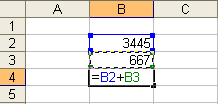 =>
=> 
Data format.
There is a need to apply different formats of data presentation.
By default, the number format is used, which displays two decimal places.
Exponential format is used if a number containing a large number of digits does not fit in a cell (for example 3500000000, then it will be written in 5.00E + 09).
Because excel program is designed to handle numbers, the correct setting of their format plays an important role. For humans, the number 10 is just one and zero. From an Excel perspective, these two numbers can convey completely different information depending on whether it represents the number of employees in a company, a monetary value, a percentage of a whole, or a portion of the "Top 10 Firms" heading. In all four situations, this number must be displayed and handled differently. Excel supports the following formats:
General (General) - assigned automatically, if the format is not specified specifically.
Number is the largest common way to represent numbers
Monetary (Currency) - monetary values
Financial (Accounting) - monetary values, aligned by the separator with integer and fractional parts
Date (Data) - date or date and time
Time - time or date and time
Percentage - cell value multiplied by 100 with% at the end
Fraction - rational fractions with numerator and denominator
Exponential (Scientific) - decimal fractional numbers
Text - text data is displayed in the same way as strings are entered and processed, regardless of their content
Additional (Special) - formats for working with databases and address lists
Custom - user-defined format
Choosing a data format
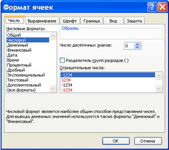
1. Enter the Format-Cell command
2. On the Format Cells dialog box, select the Number tab.
3. From the Number formats list: select the most suitable format.
 -
- 
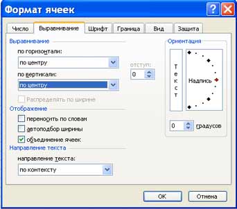
The Alignment tab is defined by:
1. Alignment - a method of aligning data in a cell horizontally (left or right, by value, center of selection, center, width, filled) or vertically (bottom or top, 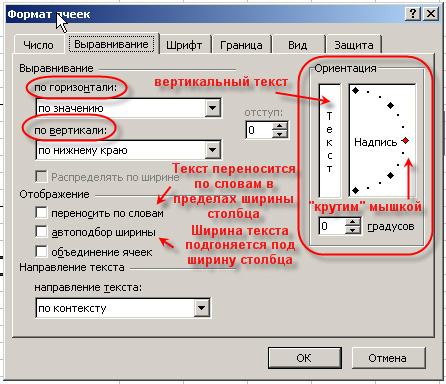 center or height);
2. Display - determines whether the text can be wrapped in a cell, according to words, enables or disables merging of cells, sets the automatic selection of the width of cells.
3. Text orientation
Font tab - changes the font, style, size, color, underline and effect of the text in the selected cells;
Border tab - creates frames (border) around the selected block of cells;
View tab - allows you to set cell shading (color and pattern);
Protection tab - controls the hiding of formulas and blocking of cells (prohibiting editing of these cells). You can set up protection at any time, but it will be effective only after the protection of a sheet or book is entered using the Service / Protect sheet command.
Entering a formula
 You can enter a formula in two ways. You can enter a formula directly into a cell or use the formula bar. To enter a formula in a cell, follow these steps:
1. Select the cell where you want to enter the formula and start writing with the "\u003d" sign. This will tell Excel that you are going to enter the formula.
2. Select the first cell or range you want to include in the formula. The address of the cell you are referring to appears in the active cell and in the formula bar.
3. Enter an operator, for example a "+" sign.
4. Click the next cell or range that you want to include in the formula. Continue typing operators and selecting cells until the formula is ready.
5. When you have finished entering the formula, click the Enter button in the formula bar or press Enter on your keyboard.
6. The cell now shows the result of the calculation. Select the cell again to see the formula. The formula appears in the formula bar.
 Another way to enter formulas is to use the Formula Bar. First, select the cell in which you want to enter the formula, and then click on the Edit Formula button (the "Equals" button) in the formula bar. The Formula Bar window appears. An equal sign will be automatically entered before the formula. Begin typing the cells you want to use in the formula and the operators needed to perform the calculations. After you have entered the entire formula, click on the Ok button. The formula appears in the formula bar, and the calculation result appears in the worksheet cell.
Often, you need to use the Function Wizard to create a formula.
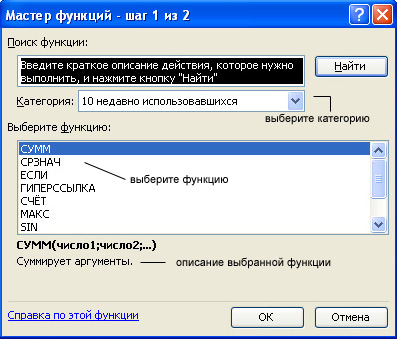 Functions can be entered manually, but Excel has a function wizard that allows you to enter them in a semi-automatic mode and with little or no errors. To call the function wizard, click the Insert function button on the standard toolbar, execute the Insert / Function command, or use a key combination. This will bring up the Function Wizard dialog box, in which you can select the desired function.
The window consists of two related lists: Category and Function. When you select one of the items in the Category list in the Function list, the corresponding list of functions appears.
When you select a function, a short description appears at the bottom of the dialog box. When you click on the ok button, you go to the next step. Step2.
Functions in Excel
To speed up and simplify computing excel work provides the user with a powerful apparatus of worksheet functions, allowing to carry out almost all possible calculations.
All in all MS Excel contains over 400 worksheet functions (built-in functions). All of them, in accordance with their purpose, are divided into 11 groups (categories):
1. financial functions;
2. date and time functions;
3. arithmetic and trigonometric (mathematical) functions;
4. statistical functions;
5. functions of links and substitutions;
6. database functions (list analysis);
7. text functions;
8. logic functions;
9. informational functions (checking properties and values);
10. engineering functions;
11. external functions.
Quest II
Spreadsheets are an electronic replacement for ledgers and a calculator. This software uses columns and rows to perform mathematical operations on previously entered data. Spreadsheets can do much more today, as they are often used as (very) simple databases or as a graphing and charting application, even though this was not the original goal of this class of software.
Figure 12.5. Rows, Columns and Cells
The lines are named like this: 1, 2, etc. The columns are named like this: A, ..., Z, AA, AB, etc. The intersection of a row and a column is called a cell, and its name is made up of the column and row attributes, for example: C3 (as shown in Figure 12.5, “Rows, Columns, and Cells”). The active row and column names are highlighted.
2.2. OpenOffice.org Calc
2.2.1. Running
To start OpenOffice.org Calc, select Office from the main menu → Spreadsheets → OpenOffice.org Calc Using office programs → Create spreadsheets... You can also open it from any other OpenOffice.org application by choosing File → New → Spreadsheet... This will open a window with a new blank OpenOffice.org Calc spreadsheet.
When you start OpenOffice.org Calc for the first time, a window will appear (see Figure 12.6, "Selecting the Default File Format")asking you which format you prefer to use for storing your files: Microsoft® or OpenOffice.org.
Figure 12.6. Selecting the default file format

Your decision depends on whether you plan to share large numbers of files with people using only Microsoft® tools. In this case, click Use Microsoft® Excel format, but we warn you that it is not perfectly supported. Also note that this is just the default format and can always be changed in the File Type field of the Save As dialog box.
2.2.2. Interface
Figure 12.7. OpenOffice.org Calc Main Window
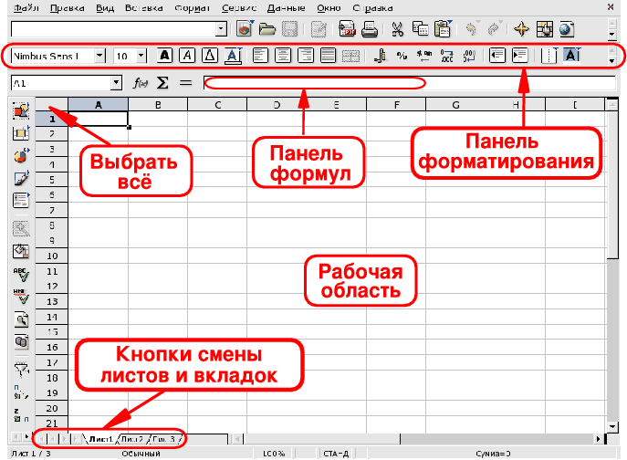
Format bar
This is a standard formatting bar used in all OpenOffice.org applications and is used to change the appearance of application data: fonts, colors, alignment, etc.
Formula barUse it to enter, edit, or delete formulas in cells.
WorkspaceThe place where you enter your spreadsheet data: numbers, dates, formulas, images, etc.
Choose allClicking on this small area in the upper left corner of the work area will simultaneously select all cells. This is useful when you need to make "global" changes to a spreadsheet. For example, set the font size in all cells to 10 points (pt).
Sheet change buttons and tabsSpreadsheet documents usually contain more than one sheet. Use these buttons to easily navigate through these sheets. From left to right: Go to the first sheet, Move to the previous sheet, Move to next sheet and Go to the last sheet. You can also use tabs to navigate through sheets.
2.3. Using spreadsheets
The following sections will cover basic functions such as entering data and formulas and adding graphs that display this data. As an example, we will use the graphs of expenses and sales for the month of an imaginary company.
OpenOffice.org Calc is a spreadsheet application for corporate and home use, and includes many features that are beyond the scope of this document. Read the section Section 2.4, “Further Study” to obtain additional information how to take full advantage of the capabilities of OpenOffice.org Calc.
2.3.1. Data input
To enter data in a cell, select this cell and enter your data by pressing the key when finished Enter . You can also use the keys Tab or Shift -Tab to move to the cell to the right or to the left, respectively.
Auto-completion simplifies data entry by "guessing" the next cell data based on the data in the current cell. This works for any data type that can be associated with a series of consecutive integers.
Figure 12.8. Simplify Data Entry with Auto-Completion

To use auto-completion, place the mouse pointer over the cell's "handle" (the small black square in the lower-right corner of the cell), click on it, and drag the cell. The cell values \u200b\u200bwill be shown in a tooltip (see Figure 12.8, “Simplifying Data Entry with AutoComplete”). After the desired final value is shown, release the mouse button and the cells will be filled.
Also, cell data can be sorted according to various criteria (in a column or row, depending on how you have arranged your data). To do this, first select the cells that you want to sort, and then open the window with sorting options by selecting the Data → Sort menu.
2.3.2. Adding formulas
Formulas can be used to "automate" spreadsheet calculations, allowing you to perform complex simulations, for example. Formulas in cells are defined by data starting with an \u003d sign. Everything else is considered "static" data.
Operations are expressed using conventionally accepted algebraic notation. For example, \u003d 3 * A25 + 4 * (A20 + C34 / B34) divides the value in cell C34 by the value in cell B34, adds A20 to the result, multiplies that by 4, and adds it to the value in cell A25 multiplied by 3. In this way, much more complex expressions can be written based on simpler expressions.
OpenOffice.org Calc provides you with many predefined functions that you can use in your formulas. View them by opening the Function Wizard from the Insert → Function menu or by pressing the keys Ctrl -F2 .
Figure 12.9, “Using a Function in a Formula” shows the AVERAGE function applied to a selected range of cells to calculate their average. Note the use of the: symbol to indicate a sequential range of cells in a function.
Spreadsheet Processors
"Spreadsheet Processors"
1. Spreadsheet Microsoft Excel
Excel is a spreadsheet processor. A spreadsheet is an application program that is designed to create spreadsheets and automate the processing of tabular data.
A spreadsheet is a spreadsheet divided into rows and columns, at the intersection of which cells with unique names are formed. Cells are the main element of a spreadsheet, into which data can be entered and referenced by cell names. Data includes numbers, dates, time of day, text or character data, and formulas.
Data processing includes:
carrying out various calculations using formulas and functions built into the editor;
building diagrams;
data processing in lists (Sorting, AutoFilter, Advanced filter, Form, Totals, PivotTable);
solving optimization problems (Selection of a parameter, Finding a solution, What-If Scenarios and Other Tasks);
statistical data processing, analysis and forecasting (analysis tools from the "Analysis Package" add-in).
Thus, Excel is not only a means of automating calculations, but also a means of modeling various situations.
Scope of Excel: planning and financial and accounting calculations, material assets accounting, decision support systems (DSS) and other areas of application.
Create a new workbook in Excel
Excel training should begin by exploring the Excel application window. When you start Excel, an application window opens and displays a new workbook - Book 1.
The Excel application window has five main areas:
menu bar;
toolbars;
status bar;
input line;
workbook window area.
The main processing of data in Excel is carried out using commands from the menu bar. The Standard and Formatting toolbars are built-in MS Excel toolbars that are located below the menu bar and contain specific sets of icons (buttons). Most of the icons are for executing the most commonly used commands from the menu bar.
The Excel Formula Bar is used to enter and edit values, formulas in cells or charts. The name field is the window to the left of the formula bar that displays the name of the active cell. The icons: X, V, fx located to the left of the formula bar are the buttons for canceling, entering and inserting a function, respectively.
The status bar of the Excel application window is located at the bottom of the screen. The left side of the status bar indicates the status information of the spreadsheet work area (Done, Enter, Edit, Specify). In addition, the results of the executed command are briefly described on the left side of the status bar. The right side of the status bar displays the results of calculations (when performing automatic calculations using the status bar context menu) and displays the pressed keys Ins, Caps Lock, Num Lock, Scroll Lock.
Next, you need to familiarize yourself with the basic concepts of the workbook window. A workbook (Excel document) consists of worksheets, each of which is a spreadsheet. By default, three worksheets or three spreadsheets open, which you can navigate to by clicking on the tabs at the bottom of the book. If necessary, you can add worksheets (spreadsheets) to the workbook or remove them from the workbook.
Tab scroll buttons scroll the workbook tabs. The outermost buttons scroll to the first and last tab of the workbook. Inner buttons scroll to the previous and next workbook tab.
Basic Spreadsheet Concepts: Column Header, Row Header, Cell, Cell Name, Selection Marker, Fill Marker, Active Cell, Formula Bar, Name Field, Active Sheet Area.
The working area of \u200b\u200ba spreadsheet consists of rows and columns that have their own names. The names of the lines are their numbers. Line numbering starts at 1 and ends with the maximum number set for this program. Column names are letters of the Latin alphabet, first from A to Z, then from AA to AZ, BA to BZ, etc.
The maximum number of rows and columns of a spreadsheet is determined by the features of the program used and the amount of computer memory, for example, in an Excel spreadsheet processor there are 256 columns and more than 16 thousand rows.
The intersection of a row and a column forms a cell in a spreadsheet with a unique address. References are used to indicate cell addresses in formulas (for example, A6 or D8).
A cell is an area defined by the intersection of a column and a row in a spreadsheet and has its own unique address.
The cell address is determined by the name (number) of the column and the name (number) of the row at the intersection of which the cell is located, for example, A10. Link - specifying the cell address.
The active cell is the selected cell whose name appears in the name field. A selection marker is a bold box around a selected cell. The fill handle is the black square in the lower right corner of the selected cell.
The active area of \u200b\u200bthe worksheet is the area that contains the entered data.
In spreadsheets, you can work with both individual cells and groups of cells that form a block. A block of cells is a group of contiguous cells identified by an address. The address of a block of cells is specified by indicating the links of its first and last cells, between which a separating character is placed - a colon. If the block looks like a rectangle, then its address is specified by the addresses of the upper left and lower right cells included in the block. The block of used cells can be specified in two ways: either by specifying the start and end addresses of the block cells from the keyboard, or by selecting the corresponding part of the table using the left mouse button.
Working with files in Excel
Saving and naming a workbook
When you save a workbook in Excel, the Save Document dialog box opens. In this window, you must specify: file name, file type, select a drive and folder in which the workbook will be stored. Thus, the workbook with its included worksheets is saved in a folder on disk as a separate file with a unique name. Book files have the xls extension.
Opening a workbook in Excel
To open a workbook in Excel, select the File / Open command or click on the Open button on the standard toolbar. Excel will display a dialog box "Open document" in it you can select the required file and click on the Open button.
Close a workbook and exit Excel
To close the workbook in Excel, select the File / Close command, which will close the workbook. To exit Excel, select the File / Exit command or click the close button on the right side of the title bar of the application window.
2. Editing and formatting Microsoft Excel worksheets
Any information processing begins with its input into a computer. In MS Excel spreadsheets, you can enter text, numbers, dates, times, sequential series of data and formulas.
Data entry is carried out in three stages:
selection of a cell;
data input;
confirmation of input (press Enter).
After the data is entered, it must be presented on the screen in a specific format. To represent data in MS Excel, there are various categories of format codes.
To edit data in a cell, double-click on the cell and edit or correct the data.
Editing operations include:
deleting and inserting rows, columns, cells and sheets;
copying and moving cells and blocks of cells;
editing text and numbers in cells
Formatting operations include:
changing number formats or the form of representation of numbers;
changing the width of the columns;
alignment of text and numbers in cells;
changing the font and color;
Selection of the type and color of the border;
Fill cells.
Entering numbers and text
Any information that is processed on a computer can be represented as numbers or text. Excel enters numbers and text by default in General format.
Text input
Text is any sequence of characters entered into a cell that cannot be interpreted by Excel as a number, formula, date, time of day. The entered text is aligned to the left in the cell.
To enter text, select a cell and type text using the keyboard. The cell can hold up to 255 characters. If you need to enter some numbers as text, then select the cells, and then select the Format / Cells command. Then select the "Number" tab and select Text from the list of formats that appears. Another way to enter a number as text is to enter an apostrophe before the number.
If the text does not fit into the cell, then you need to increase the column width or allow word wrap (Format / Cells, Alignment tab).
Entering numbers
Numeric data are numeric constants: 0 - 9, +, -, /, *, E,%, period and comma. When working with numbers, you must be able to change the type of entered numbers: the number of decimal places, the type of the integer part, the order and sign of the number.
Excel independently determines whether the information entered is a number. If the characters entered into the cell refer to text, then after confirming the entry into the cell, they are aligned to the left edge of the cell, and if the characters form a number, then they are aligned to the right edge of the cell.
Consecutive data entry
Data series means data that differ from each other by a fixed step. However, the data does not have to be numeric.
To create data series, you need to do the following:
1. Enter the first term of the series into the cell.
2. Select the area where the row will be located. To do this, move the mouse pointer to the fill marker, and at this moment, when the white cross turns into black, press the left mouse button. Further, while holding down the mouse button, you need to select the desired part of the row or column. After you release the mouse button, the selected area will be filled with data.
You can build a data series in another way, if you specify a build step. To do this, you need to manually enter the second term of the series, select both cells and continue the selection to the desired area. The first two cells, entered manually, set the step of the data series.
Data format
Data in MS Excel is displayed in a specific format. By default, information is displayed in General format. You can change the presentation format of the information in the selected cells. To do this, run the Format / Cells command.
The "Format Cells" dialog box appears, in which you need to select the "Number" tab. On the left side of the "Format Cells" dialog box, the "Number Formats" list contains the names of all formats used in Excel.
For the format of each category, a list of its codes is provided. In the right window "Type" you can view all format codes that are used to represent information on the screen. For data presentation you can use built-in MS Excel format codes or enter your (custom) format code. To enter a format code, select a line (all formats) and enter the format code characters in the "Type" input field.
Data presentation style
One way to organize data in Excel is to introduce style. To create a style, use the Format / Style command. Execution of this command opens the "Style" dialog box.
3. Technology of creating a spreadsheet
Let us consider the technology of creating a spreadsheet using the example of designing the Inventory Accounting table.
1. To create a table, execute the File / New command and click on the Blank Book icon in the task pane.
2. First, you need to mark up the table. For example, the Goods Accounting table has seven columns, which we assign to columns from A to G. Next, you need to form the table headings. Then you need to enter the general title of the table, and then the names of the fields. They must be on the same line and follow each other. The header can be positioned in one or two lines, aligned to the center, right, left, bottom or top of the cell.
3. To enter the title of the table, place the cursor in cell A2 and enter the name of the table "Remains of goods in the warehouse".
4. Select cells A2: G2 and execute the Format / Cells command, on the Alignment tab, select the center alignment method and check the box for merging cells. Click OK.
5. Creation of the "header" of the table. Enter the names of the fields, for example, Warehouse No., Supplier, etc.
6. To arrange the text in the cells of the "header" in two lines, select this cell and execute the Format / Cells command, on the Alignment tab, check the Wrap by words box.
7. Insert different fonts. Select the text and select the Format / Cells command, the Font tab. Set the typeface, for example, Times New Roman, its size (point size) and style.
8. Align the text in the "header" of the table (select the text and click on the Center button on the formatting toolbar).
9. If necessary, change the width of the columns using the Format / Column / Width command.
10. You can change the line heights using the Format / Line / Height command.
11. Adding a frame and filling of cells can be done by the Format / Cell command on the Border and View tabs, respectively. Select the cell or cells and on the Border tab select the line type and use the mouse to indicate to which part of the selected range it belongs. On the View tab, select a fill color for the selected cells.
12. Before entering data into the table, you can format the cells of the columns under the "header" of the table using the Format / Cells command, Number tab. For example, select the vertical block of cells under the cell "Warehouse number" and choose Format / Cells on the Number tab, select Numeric and click OK.
List of references
Electronic student, - "Formulas, functions and charts in Excel" lessons-tva / call date: 05.11.10
Similar abstracts:
Practical use of Excel. Assignment of commands and their execution. "Freeze areas", a new workbook and its saving, lists and their use in data entry. Inserting notes. Auto-formatting tables. Protection of sheets and books. Building diagrams.
The main elements of spreadsheets in MS Excel and techniques for working with them. Types of variables, ways of formatting cells. Create, save and rename a workbook. Range of cells and their automatic selection. Number and currency formats of cells.
Information processing in Excel spreadsheets or lists, basic concepts and requirements for lists, economic and mathematical Excel applications. Solution of equations and optimization problems: selection of parameters, "Search for a solution" command, scenario manager.
The working area of \u200b\u200bthe window and the structure of MS Excel. Application and capabilities of spreadsheets, the benefits of using when solving problems. Entering and editing data in cells, copying data, building diagrams, professional paperwork.
Formulas as an expression consisting of numerical values \u200b\u200bconnected by signs of arithmetic operations. Excel function arguments. Using formulas, functions and charts in Excel. Entering functions in a worksheet. Creation, assignment, placement of chart parameters.
Microsoft file Excel is a workbook. The data can be numbers or text. Data input. Selection of cells. Removing information from cells (from a group of cells). Work with workbooks. Removing a sheet. Renaming sheets. Saving the file.
Sorting the source data by the average stock for the quarter. The sum of the average stock for the quarter for all objects. Distribution of control objects into groups. Plotting the ABC Curve with the Chart Wizard. Solving the XYZ problem in parallel with the ABC analysis.
Ways to start Excel and exit it, general rules work with the program and its main functions. The order of inserting rows, columns and sheets, combining cells. Copying and moving data within one sheet. Protection and printing of sheets and books.
You can save time when creating a SharePoint list by importing a spreadsheet file. When you create a list from a spreadsheet, its column headings in the list become, and the rest of the data is imported as list items. Importing a spreadsheet is also a way to create a list without a default column header.
Important:
Important: If you receive a message stating that the spreadsheet that you want to import is invalid or does not contain data, add the SharePoint site with which you are listed on the Trusted Sites tab.
Create a spreadsheet-based list in SharePoint Online 2016, and 2013
On the search results page, click Importing a spreadsheet.

On the page New app enter name list.

Enter description (not necessary).
The description appears under the name in most views. The description of the list can be changed in its parameters.
Click the button Overviewto find the spreadsheet, or enter the path to it in the field File location... When finished, click Import.
The spreadsheet will open in Excel and a window will appear.
In the window Import to Windows SharePoint Services List select item Table range, Range of cells or Named range... If you want to specify the range manually, select Range of cells and click Select a range... In the spreadsheet, click the top-left cell, press and hold the SHIFT key, and select the bottom-right cell in the range.

The range will be indicated in the field Select a range... Click the button Import.
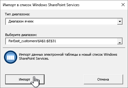
List or click the Options button and click List options.
The table data appears as a list in SharePoint.
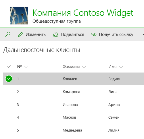
On the site where you want to add the list, click Options and select Add application.
In field Find app enter "spreadsheet" and click the search icon.

Create a list from a spreadsheet in SharePoint 2010 or SharePoint 2007
On the menu Site actions
 select team View all site content and press the button Create a
.
select team View all site content and press the button Create a
.Note: SharePoint sites can look different. If you cannot find an item, such as a command, button, or link, contact your administrator.
In SharePoint 2010 under All categories click Blank and custom, select and click Create a.
In SharePoint 2007, under Customizable lists select Import spreadsheet and press the button Create a.

Enter a name for the list in the box Name... Field Name is required.
The name appears at the top of the list in most views, becomes part of the web address of the list page, and appears in navigation controls for easier search. You can change the name of the list, but the web address remains the same.
Enter a description for the list in the box Description... Field Description is optional.
The description appears under the name in most views. The description of the list can be changed.

Click the button Overviewto select a spreadsheet, or enter the path to it in the field File locationand then click Import.
In the dialog box Import to Windows SharePoint Services List select Range typeand then in the section Select a range specify the range in the spreadsheet that you want to use to create the list.
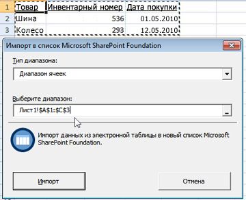
Note: In some spreadsheet editors, you can select the desired range of cells directly in the spreadsheet. The table range and the named range must already be defined in the table to be selectable in the dialog Import to Windows SharePoint Services List.
Click the button Import.

After importing the spreadsheet, check the list columns to make sure the data was imported correctly. For example, you might want to specify that a column contains monetary values, not numbers. To view or change the options for a list, open it, go to the tab List or click the Options button and click List options.
The column types that are created for the list are based on the data types in the columns in the spreadsheet. For example, a column in a spreadsheet that contains dates usually becomes a date column in a SharePoint list. The figure below shows a SharePoint list that was created by importing the above spreadsheet.
All versions of SharePoint support importing spreadsheets, but the steps are slightly different. These examples used Excel, but another compatible editor will work as well. If the spreadsheet editor format is not supported, export the data to a comma-delimited (CSV) file and import the file.
For links to articles on customizing an imported list and adding it to a page or site, see Understanding Lists.
Note: Typically, columns in a SharePoint site are configured based on the type of data they contain. However, after importing the list, check the columns and data to make sure the import was correct. For example, you might want to specify that a column contains monetary values, not numbers. To view or change the options for a list, open it, and then click List options on the menu Options.
Add a site to the Trusted sites zone
Open the Internet Explorer browser, click the button Service and select item Internet Options.
Go to the tab Security, click the icon Reliable nodes and press the button knots.
You are on the site will be displayed in Add this website to the zone: fields, click Add to.
Click the button Close, and then - Ok.
Leave a comment
Was this article helpful? If yes, please leave your feedback at the bottom of the page. Otherwise, share your opinion - what needs to be added or made clearer. Please include your SharePoint version, OS and browser. We will read your feedback, double-check the information and, if necessary, add and update this article.
Note: Disclaimer regarding machine translation... This article was translated using a computer system without human intervention. Microsoft offers these machine translations to help users who don't know of English language, read materials about Microsoft products, services, and technologies. Since the article was translated using machine translation, it may contain lexical, syntax and grammatical errors.