Addition formulas in Excel. Functions in Microsoft Excel. The formula of spent days.
17.03.2017
Many users are aware of the Excel spreadsheet processor. Someone installed it just to open tables, and someone - to compose them. Often, when entering data into a table, you may need a calculator to calculate rather large numbers. So to save our time, the addition function (subtraction, multiplication and subtraction) was built into Excel. However, not everyone knows how to apply it. This is what will be discussed in the article.
Calculates interest on unified depreciation payments for investments. Interest is the interest rate for the period. Period is the number of periods to calculate interest. Investment is the value of an investment. Monthly interest rate after 1, 5 years is 300 units of currency.
Returns the internal rate of return for an investment. Numeric values \u200b\u200brepresent cash flows coming in at regular intervals, with at least one negative value and at least one positive value. Values \u200b\u200bis an array containing values.
How to calculate the amount in a column
In fact, there are several ways to add numbers in a column, and we will consider all of them in detail. But first, let's take any table as an example.
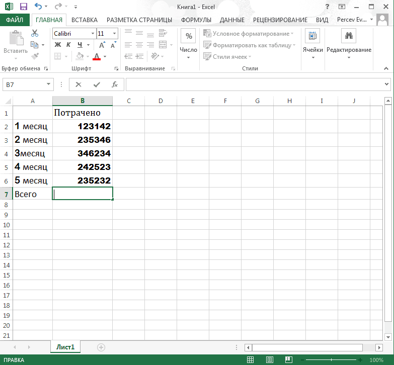
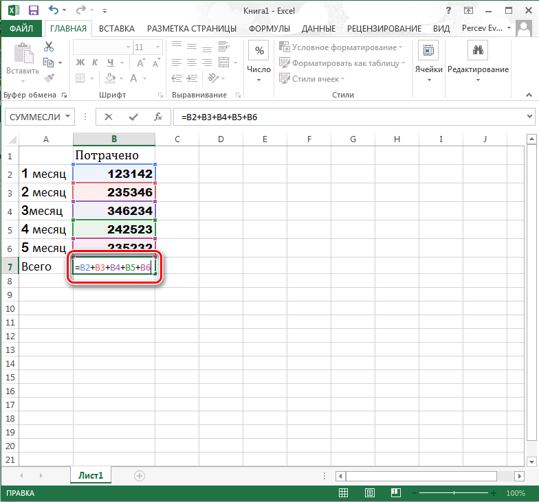
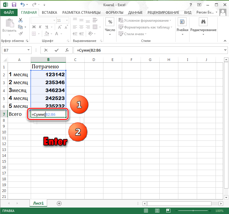
Method 1: Entering cells
Let's assume this is an approximate value for the result. The internal rate of return is calculated using the iterative method. If you can only give a few values, you should establish an initial guess on which the iterations are based.
Returns the actual annual interest rate up to the specified nominal annual interest rate. The nominal interest rate is the interest payable at the end of the period under review. The actual interest rate increases with the number of payments made. In other words, interest is often paid in installments until the end of the period.
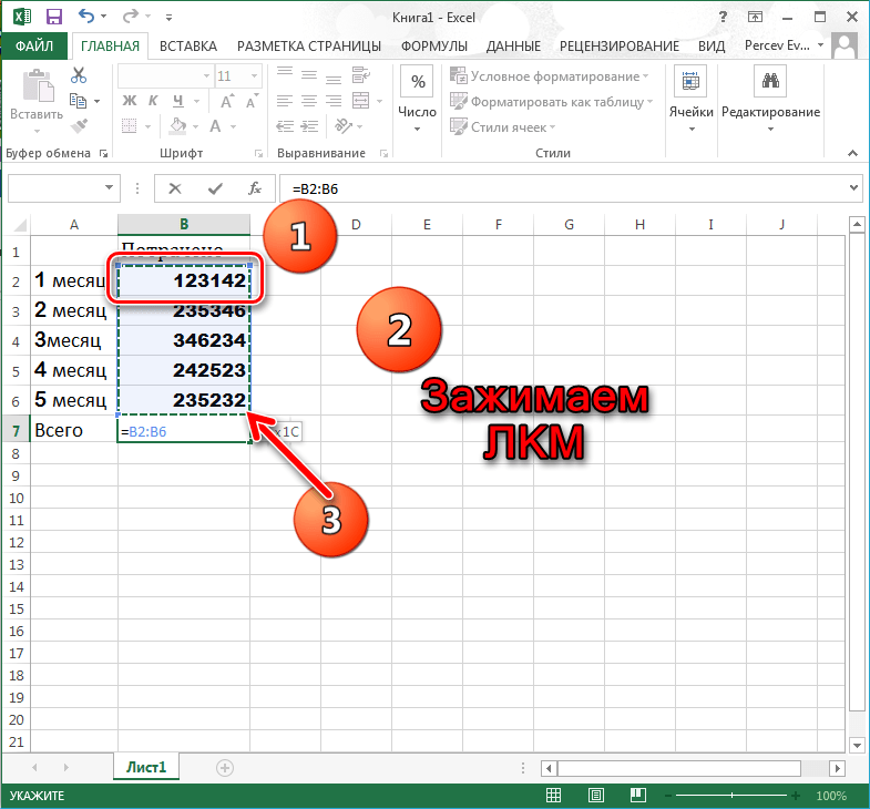
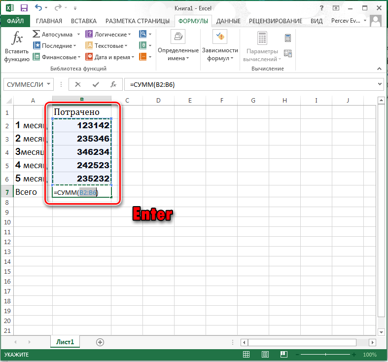
Method 2: Select a column
This method is similar to the previous one. But this one will be much easier, since the formula will be entered by itself.
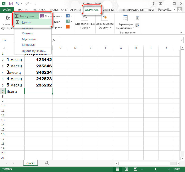
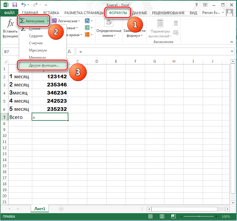
Method 3: "AutoSum" department
This method is different from all the others, since here you will need to access the Quick Access Toolbar.
If the nominal annual interest rate is 9.75% and interest is paid four times a year, what is the actual interest rate? Returns the actual annual interest rate based on a given nominal annual interest rate and number of interest periods per year.
What is Excel?
Nominal nominal interest rate. What is the actual annual interest rate at a nominal interest rate of 5, 25% and quarterly payments? Calculates the duration in years of a fixed interest rate. The transaction is the date of purchase of the security.
Method 4: "SUMIF" function
Another helper function with which you can set the summation conditions.
Now you have learned about such opportunities table processor Excel as summing numbers in a column. This knowledge can be applied during the preparation of protocols and reports, and when entering ordinary data.
Maturity is the maturity of the guarantee at the end of its validity period. Coupon is the annual percentage rate of the security coupon. The yield is the annual yield of the collateral. Frequency is the number of coupon payments per year. The basis is selected from several fixed options and indicates how to calculate the year.
The nominal interest rate is 8%. Interest is paid for six months. If we use the daily balance, how much is the modified duration? Returns the security discount rate as a percentage. The price is the price of the book per 100 units of par value currency.
The SUM function belongs to the category: "Mathematical". Press the SHIFT + F3 hotkey combination to invoke the function wizard, and you will quickly find it there.
Using this function significantly expands the capabilities of the process of summing the values \u200b\u200bof cells in excel program... In practice, we will consider its capabilities and settings when summing several ranges.
Potential is the cost of paying out a book for 100 face value units. The purchase price is 97 and the redemption value. If daily balancing is used, what is the discount rate? Calculates the depreciation of an asset over a specified period using the arithmetic degressive method.
Autosum for multiple columns
This calculation method is suitable if you want a higher initial depreciation compared to the straight-line method. The amortized cost decreases with each successive period - this is usually the case for assets that depreciate most quickly after purchase. Note that in this method, the residual value cannot reach.
How to calculate the sum of a column in an Excel spreadsheet?
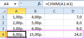
Let's sum up the value of cells A1, A2 and A3 using the sum function. For one thing, we'll find out what the sum function is used for.
As a result, the result of the calculation is displayed in cell A4. The function itself and its parameters can be seen in the formula bar.
Note. Instead of using the "Sum" tool on the main panel, you can directly enter a function with parameters manually in cell A4. The result will be the same.
The term is the number of periods of the asset's useful life. Period is the period for which the value is calculated. Coefficient - the coefficient of the balance reduction. If no value is entered, it is assumed. The value at the end of the depreciation period is 1 currency.
Summarizing data and considering them from different points of view
Calculates the depreciation of an asset for the selected period using the fixed residual depreciation method. This calculation method is used when you want to get higher depreciation at the beginning of the asset's life. The depreciation value is reduced in each subsequent period by the total depreciation for the previous periods.
Correction of automatic range recognition
When entering a function using a button on the toolbar or when using the function wizard (SHIFT + F3). the SUM () function belongs to the group of formulas "Mathematical". The auto-recognized ranges are not always user-friendly. They can be quickly and easily corrected if necessary.
Liquidity is the residual value of an asset at the end of the depreciation period. Period is the length of periods. It must be in the same units as the depreciation period. Month defines the number of months in the first year of the depreciation period. If not set, it is implied.
Calculates depreciation for the reporting period using the straight line method. If the asset is acquired during the reporting period, the proportionate portion of the depreciation is taken into account. The rate is the rate of depreciation. Calculates depreciation for the reporting period using the degressiveness method.
Assessed value is the value of an asset. First period - the end date of the first reporting period. A period is the reporting period for which it was calculated. Returns the accrued interest for a security that pays interest on maturity.
Let's say we need to sum several ranges of cells, as shown in the figure:
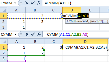
- Go to cell D1 and select the Sum tool.
- While holding down the CTRL key, additionally select the range A2: B2 and cell A3 with the mouse.
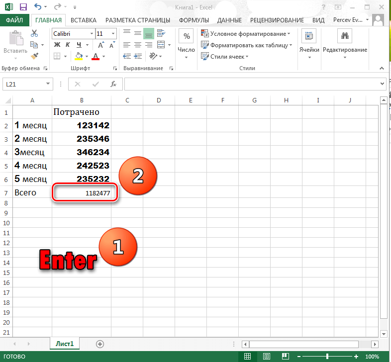
- After selecting the ranges, press Enter and in cell D4 the result of summing the values \u200b\u200bof the cells of all ranges will immediately appear.
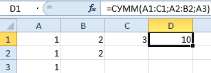
Pay attention to the syntax in the function parameters when selecting multiple ranges. They are separated from each other (;).
Add values \u200b\u200bin a range based on one condition using a single function or a combination of functions
Returns the accrued interest on a security that pays interest periodically. The transaction is the date on which the accrued interest is to be calculated. The interest rate is the annual percentage rate of the security coupon. The par value is the par value of the collateral.
Interest is paid twice a year. The basis is based on the American method. You can refer to the area of \u200b\u200badjacent cells by entering the coordinates of the area's top-left cell, followed by a colon, and the coordinates of the area's bottom-right cell. Absolute references are the opposite of relative addressing.
The parameters of the SUM function can contain:
- links to individual cells;
- references to ranges of cells, both contiguous and non-contiguous;
- whole and fractional numbers.
In function parameters, all arguments must be separated by semicolons.
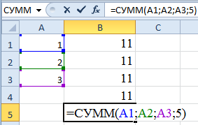
For illustrative example Consider different options for summing cell values \u200b\u200bthat give the same result. To do this, fill in cells A1, A2 and A3 with the numbers 1, 2 and 3, respectively. And fill in the range of cells B1: B5 with the following formulas and functions:
When to use relative and when to use absolute links
How are relative links different? Line numbers are also automatically adjusted when a new line is inserted. However, be careful when copying the formula, as it only redirects relative references, not absolute references. Absolute inversions are used when a calculation cites a specific cell from a worksheet. If a formula citing that cell is copied to the cell below the original, the address will also be moved down unless you set the cell coordinates to absolute.
- \u003d A1 + A2 + A3 + 5;
- \u003d SUM (A1: A3) +5;
- \u003d SUM (A1; A2; A3) +5;
- \u003d SUM (A1: A3; 5);
- \u003d SUM (A1; A2; A3; 5).
In any case, we get the same calculation result - the number 11. Consecutively move the cursor from B1 to B5. In each cell, press F2 to see the colored highlighting of the links for a clearer analysis of the syntax of writing function parameters.
Except when new rows and columns are inserted, links can also be changed when existing formulawho quotes certain cells, is copied to another area of \u200b\u200bthe sheet. If you want to calculate the sum of the adjacent column to the right, just copy this formula into the cell to the right.
Summarizing is an essential part of data analysis, whether you're looking for Northwest Interim Sales or Weekly Total Sales. To help you do the best choiceThis article provides a complete summary of the methods that support information to help you quickly decide which method to use, and links to more detailed articles.
Simultaneous column summation
In Excel, you can sum multiple contiguous and non-contiguous columns at the same time.
Fill in the columns, as shown in the picture:
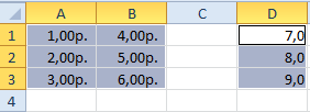
- Select the range A1: B3 and while holding down the CTRL key also select the column D1: D3.
- On the Home panel, click the Sum tool (or press ALT + \u003d).
Note. This function automatically substitutes the format of the cells that it sums up.
Collect values \u200b\u200bin a cell using a simple formula
Under Number of Cells, Rows, or Columns. You can collect and subtract numbers using simple formulaby pressing the button or using the sheet function. Do it with a plus sign using the arithmetic operator.
Remove values \u200b\u200bin a cell using a simple formula
Do it with the minus sign using the arithmetic operator. For example, the formula \u003d 12-9 shows the result.Collect values \u200b\u200bin a column or row using the button
Click an empty cell under the column of numbers or to the right of the row of numbers, and then click Startup.