How to create a table in Excel video. Training in Excel.
The Excel program is a multifunctional application, the functionality of which clearly exceeds the ability to any other. Without this application, do not do economists, accountants, etc. specialists. Excel allows you to draw all sorts of graphics, tables, etc., which greatly simplifies life.
Nevertheless, despite the huge number of functions, the tables are still the most basic function used by users. It is because of the need to draw a beautiful table, say, for a presentation or for work, many download Excel and, of course, do it right. After all, this program is perfectly sharpened to perform such actions, and the tables may have all sorts of shapes and sizes and, moreover, very simple! But let's go about everything in order. So, then we will discuss how to make tables in Excel.
How to draw a table in Excel
How to work with a table
Now you can adjust the table itself, change / add data, delete / add lines and columns, thereby expanding the borders of the table, etc. For example, if you hover the cursor to the lower corner of the table and pull it out for it, it will begin to increase, it is also possible to achieve its reduction.
The table can be done a little daily. To do this, highlight any line or column and click the right mouse button on it. A menu will fall out in which you want to select "Paste", and then - any of the listed lines, for example, "Columns of the table on the left". In this way, your plate can turn all new elements. Also, according to the table, you can. I hope that the question is how to work with tables in Excel has become more understandable for you! 
Of course, all the nuances will not consider it, there are many of them. But the most basic, so to speak, the basics, you now know, and then it's small - draw the table yourself!
Video to help
In this lesson you will learn how to create tables in Excel 2010, and you will learn how to edit tables in Excel 2010, learn how to select the style you need for your Tables Excel 2010.
And so let's start creating a table in Microsoft Excel. 2010.
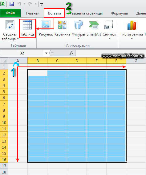
To create a table in Excel 2010 you need to highlight the cell with which your table will begin. For example: Mouse over one of the cells on one of the cells and press the left mouse button once (for example, we take the B2 cell) after the actions were performed cell B2 will become active.
1.
Now hover the mouse over the active cell and press the left mouse button and, without releasing the left mouse button, pull the mouse cursor to the bottom and right to the length you need and the width.
2.
Now that you have an approximate table in Excel 2010, you need to select the "Insert" tab, then click on the "Table" button.
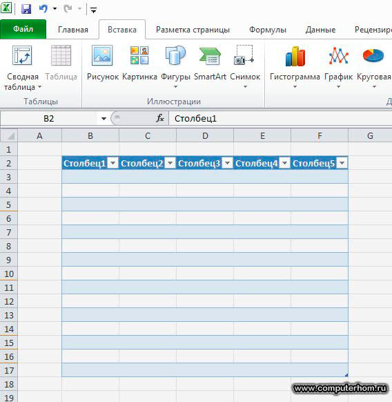
When you click on the "Table" button, the window in Excel 2010 will open the window in which the length and width of your table will be specified, there is nothing in this window and click on the "OK" button.

When you click on the "OK" button, a table will appear in the Excel 2010 book. Now you can proceed to edit the table (table formatting).
When you have a table in Microsoft Excel 2010, then you will have an optional Designer tab in the Microsoft Excel 2010 panel, with which we will be able to edit our table.
If you have an additional tab "Designer" on your toolbar, then in the created table, do at least one active cell, then an additional tab "Designer" appears on the Microsoft Excel 2010 panel.
And we will proceed to format the table, on the Microsoft Excel 2010 panel, select the Designer tab, then on the right side of Microsoft Excel 2010 you will see additional "table styles" functions, in which we now choose one style for our table.
To select the style for our table in the additional "table styles" features, press the left mouse button on the down arrow button.
Excel program is needed in order to make tables and make calculations. Now we will learn to properly compose and issue tables.
Open Excel (Programs - Microsoft Office - Microsoft Office Excel).
At the top are the editing buttons. Here's what they look at Microsoft Excel 2003:
And so - in Microsoft Excel 2007-2016:
After these buttons is the working (basic) part of the program. It looks like a large table.
Each cell is called a cell.
Pay attention to the uppermost cells. They are highlighted in different color and are called A, B, C, D, and so on.
In fact, it is not a cell, but the names of the columns. That is, it turns out, we have a column with cells a, a column with cells B, a column with C cells and so on.
Also pay attention to small rectangles with numbers 1, 2, 3, 4, etc. On the left side of the Excel program. This is also not a cell, but the names of the lines. That is, it turns out, the table can also be divided into strings (string 1, line 2, line 3, etc.).
Based on this, each cell has a name. For example, if I click on the first top cell on the left, then we can say that I clicked on the cell A1, because it is in the column A and in line 1.

And the next picture is pressed B4 cell.
Note when you click on a particular cell, then the column and the string in which they are located, changes color.
And now let's try to print a few numbers in B2. To do this, click on this cell and on the keyboard to dial numbers.
To secure the entered number and go to the next cell, press the ENTER button on the keyboard.
By the way, cells, rows and columns in Excel are very and very much. You can fill in the table at least to infinity.
Design buttons in Excel
Consider the design buttons at the top of the program. By the way, they are in Word.
Font. What style will be written text.
Size letters
Inscription (bold, italic, underlined)
Using these buttons, you can align text in the cell. Put it on the left, centered or right.
By clicking on this button, you can cancel the previous action, that is, to return back to one step.
Changing the color of the text. To select a color, you need to click on the small button with the arrow.
With this button you can paint the cell. To select the color you need to click on the small arrow button.
How to make a table in Excel
Look at the already compiled in Excel small table:
Its upper part is a hat.
In my opinion, make the cap is the hardest in the design of the table. You need to think over all items, much to provide. I advise you to take it seriously, because very often due to the wrong hatch you have to redo the entire table.
Behind the cap follows content:
And now in practice, we will try to draw up in excel program Such a table.
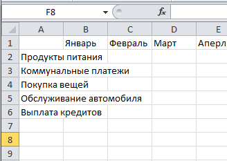
In our example, the hat is the top (first) string. Usually she is there and is located.
Click on the A1 cell and type the first item "Name". Then click in the B1 cell and type the following item - "Quantity". Please note that words are not placed in cells.
![]()
Fill out the remaining C1 and D1 cells.
![]()
And now we give a cap in a normal look. First you need to expand the cells, or rather the columns in which words did not fit.
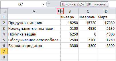
To expand column You need to bring the cursor (arrow of the mouse) to the line, separating two columns, in our case the line between A and V. The cursor will change and takes the appearance of an unusual two-sided black arrow. Click the left mouse button and, without releasing it, stretch the column to the desired width.

The same can be done with lines.
For string expansion Mouse over the line for a line that shares the two lines. The cursor will change and take the appearance of an unusual bilateral arrow of black. Press the left mouse button and, without releasing it, stretch the string to the desired width.

Expand the columns in which the text did not fit. Then slightly zoom in the header. To do this, move the cursor over the line between the line 1 and 2. When it changes the view, press the left button and, without releasing it, expand the first string.
It is accepted that the hat is somewhat different from the contents. In the table that we repeat, the chapter points "thicker" and "black" than the rest of the contents, as well as the cells are painted with gray. To do this, you need to take advantage top Excel programs.
Press the A1 cell. With this simple action, you will highlight it, that is, "say" the Excel program that you are going to change something in this cell. And now press the button at the top of the program. The text in the cell will be thicker and black (bold).
Of course, the remaining items can be changed in the same way. But imagine that we are not four of them, and forty-four ... a lot of time it will take it. To make it faster, you need to highlight the part of the table that we are going to change. In our case, this is a hat, that is, the first line.
There are several methods of selection.
Allocation of all excel tables . To do this, click on a small rectangular button in the left corner of the program, above the first string (rectangle with a number 1).
Selection of part of the table. To do this, click on the cell with the left mouse button and, without releasing it, circle the cells that you need to highlight.
Selection of column or string. To do this, click on the name of the desired column
or string
By the way, in the same way you can select several columns, rows. To do this, click on the name of the column or the lines with the left mouse button and, without releasing it, pull in columns or rows that you want to highlight.
Now let's try to change the cap of our table. To do this, highlight it. I propose to highlight the string entirely, that is, click on the figure 1.
After that, let's make letters in the cells thicker and black. To do this, press the button
Also in the table that we need to do, the words in the header are located in the center of the cell. To do this, click
Well, finally, the cells in the cap light gray. To do this, use the button.
To choose suitable color, Click on the small button next to the colors that appeared to select the desired one.
The most difficult we did. It remains to fill in the table. Do it yourself.
And now the last touch. Change the font and size of letters in the entire table. Let me remind you that for a start we need to highlight the part we want to change.
I propose to highlight the entire table. To do this, click
Well, and change the font and the size of the letters. Click on the small button with the arrow in the field that is responsible for the font.
From the list that appears, select some font. For example, ARIAL.
By the way, fonts in programs from Microsoft Office set are very many. True, not all of them work with the Russian alphabet. Make sure that there are many of them, by clicking on the small button with an arrow at the end of the field to select the font and srolling the wheel on the mouse (or moving the slider on the right side of the window that appears).
Then change the size of the letters. To do this, click on the small button in the size field and select the desired (for example, 12) from the list. I remind you that the table must be highlighted.
If suddenly letters stop fit into cells, you can always expand the column as we did at the beginning of the table.
And one more very important point. In fact, the table compiled by us will be without boundaries (without partitions). It will look like this:
If you are not satisfied with such a "unlimited" option, you must first highlight the entire table, then click on the small arrow at the end of the button that is responsible for the borders.
From the list, select "All Borders".
![]()
If you are all done correctly, then this is such a table.
Good day, dear reader of my site. I have not written new articles for a long time, and I still decided. The topic "" is quite complicated for development, but useful if you deal with a large number of numbers. What I will show in this article.
This lesson will be devoted to the main purpose of spreadsheets. And if possible, I will tell you how to make a table with calculations and plus to this table to build a schedule. I hope the article will be useful and interesting.
1. Basic table management elements.
2. Building a table.
3. Editing table and filling data.
4. Use of formulas in Excel.
5. How to make a schedule in Excel.
6. General design Document.
7. We draw conclusions.
Basic table management elements.
In the last lesson, we studied the structure of the sheet of spreadsheets. Now let's try to apply some controls in practice.
Write a table header.
There are three options here. The first option without combining cells. The second option using the cell combining tool. And the third option is to insert the element of the figure in which you insert the text of the header.
Since we need to learn how to work professionally and efficiently in Excelpro, forget forever. Why? This is not correct, not professionally and with further work there may be many problems when editing and mapping.
Personally, I use the second or third option. Ideally, if you learn how to use the elements of the shapes and insert the text in them. It is forever forget about the problem of placing the text and its further editing and adjustment.
Consider how this is done:
1. Select the right mouse button area of \u200b\u200bthe cells that we need to combine. To do this, put the mouse cursor in the first cell of the area and keeping the left mouse key lead to the final cell area.
2. In the toolbar - Tab Main - Block Alignment - Tool Combine cells. Choose the parameter you need and click on it.
Watch Figure: 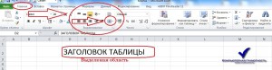
3. Click on the combined cell twice the left mouse button and enter the header text. It can also edit, change the size, font style and alignment in cells.
Building a table.
Go to the next item, building a table. Use the selection of cells, select the area you need and set the border of the table. To begin with, draw schematically on a sheet of paper or in the head (if you can imagine visually) table structure. The number of columns and lines. And then, already proceed to the allocation of the area. It will be easier.
Watch Figure: 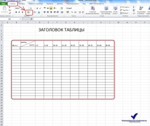
Tab Home - Block Font - Border Tool. Select the desired version of the distinguished boundaries. In my case - all borders.
You can also set the thickness of the border allocation line, the color of the lines, the style of the lines. These elements give a more elegant, and sometimes understandable to the readable form of the table. We will talk about it in more detail later in the chapter "Registration of the document".
Editing table and filling data.
And now the most responsible moment you need to remember. Editing tables is as follows.
1) We highlight the desired area. To do this, first we determine what will be in the cells. It may be numbers that denote money equivalent, interest, measuring values, or simple numbers.
2) Click on the highlighted area with the right mouse button and in the context menu, select the item "Format of the cells ..."
3) Deciding with a digital value, choose the display format you need.
Watch Figure: 
4) Configure automatic alignment of cell content. Here you optimally choose: to transfer the width according to or auto production.
Watch Figure: 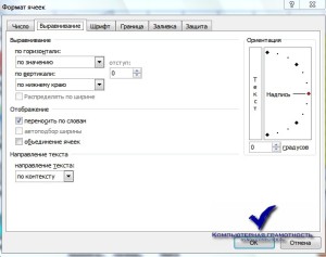
This is an important point that will help you to watch in the cells of the number as numbers, and the cash equivalent as a cash equivalent.
Use of formulas in Excel.
Go to the main part, which will consider the full potential of spreadsheets.
Let's start with the automatic numbering of cells. We put the digit "1" in the first cell, the number "2" into the second cell. We highlight these two cells. In the lower right corner of the boundary of the selected area, click on a small black square. Holding the left mouse button, pull in the direction of the numbering, thereby continuing to highlight the column or string. In the desired cell, you stop and let go of the mouse.
Watch Figure: 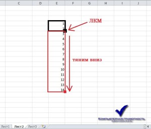
This feature allows you to apply distribution and copy to selected cells.
Formula of addition, subtraction, multiplication, divisions.
In order to make any computation, you must enter the value "\u003d" in the cell. Next, the mouse cursor click on the cell with the first indicator, set the calculation sign and click on the second indicator, and at the end of the calculation, press the Enter key.
Watch Figure: 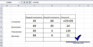
The "sums" function is required for summation a plurality of cells. Type of formula Next: \u003d sums (amount range)
Watch Figure: 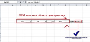
We put the cursor in the brackets and the cursor allocate the summable area.
Here are the basic formulas that are most often found in working with spreadsheets. And now the task: you need using these formulas, make a touch table.
Watch Figure: 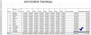
Who does not work out in the comments, I will help!
How to make a schedule in Excel.
Creative moment in this lesson, stepped! What is a diagram? This is a graphic, visual display of data in the form of two scales of indicators and results.
To build a chart, we need a table in which there are at least two indicators.
We see an example: 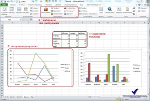
And look at the chart formatting
1) Designer 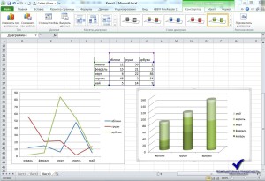
2) Layout 
3) format 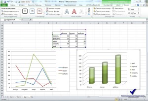
In these three tabs, you will find everything you need for quality design chart. For example, the name of the axes, the header of the chart, appearance.
Ready to task?
To the table you executed in the previous task you need to build a chart.
You can have your own option! At the end of the article, I will show my own.
General design document.
Design of spreadsheets, as well as any text document It is necessary to give a style. The style in turn can be a business, draft, presentation, educational, youth.
This section can include the following points:
- Color allocation.
- Use of various fonts.
- Location of objects in the document.
- Registration of charts and other objects.
All these items are primarily aimed at the fact that anyone could easily understand all the values \u200b\u200band indicators. As well as a beautiful or strict appearance of the document, depending on the destination, should emphasize your competence and professionalism.
We look at my design option: 
Of course, not the most original and best, but emphasizing everything that can be applied to design.
We draw conclusions.
The material in the article can be said huge. But at the same time, I tried to highlight all moments that reveal the potential and appointment of spreadsheets. I gave the basic tools for the full use of spreadsheets for the purpose.
At first glance it seems, very increasingly and insurmountable. But it is not so! Take a similar table and schedule at the rate of your cash per month or week. Or, for example, make calculation of your travel trips. Thus, you will get the statistics and analytics tools.
I will be glad if you knock on the social buttons a couple of times and leave comments to my hard work.
See you in the following articles!
Within the first Excel 2010 material for beginners, we will get acquainted with the basics of this application and its interface, learn how to create spreadsheets, as well as enter, edit and format the data in them.
Introduction
I think I will not be mistaken if I say that the most popular application included in the Microsoft Office package is a test editor (processor) Word. However, there is another program, without which any office worker rarely cost. Microsoft Excel (Excel) refers to software products called spreadsheets. FROM using Excel, in a visual form, you can calculate and automate the calculations of almost all anything, starting with a personal monthly budget and ending with complex mathematical and economic and statistical calculations containing large amounts of data arrays.
One of the key features of the spreadsheet is the ability to automatically recalculate the value of any desired cells when changing the contents of one of them. To visualize the data obtained, on the basis of groups of cells, you can create different kinds charts consolidated tables and cards. In this case, the spreadsheets created in Excel can be inserted into other documents, as well as save in a separate file for subsequent use or editing.
To call Excel simply the "spreadsheet" will be somewhat incorrect, as there are huge opportunities in this program, and in its functionality and the circle of solved tasks, this application, perhaps, can exceed Word. That is why, within the framework of the Excel materials cycle for beginners, we will get acquainted with the key capabilities of this program.
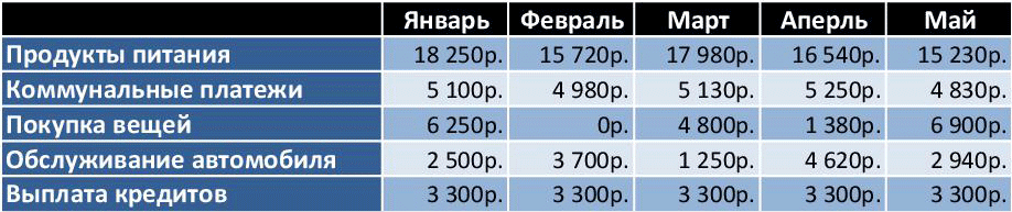
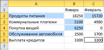
Now, after the end of the introductory part, it's time to move on to business. In the first part of the cycle, for better assimilation of the material, as an example, we will create a conventional table, reflecting personal budget expenditures for six months of this type:
But before starting it to create it, let's first consider the basic elements of the interface and control of Excel, as well as let's talk about some basic concepts of this program.
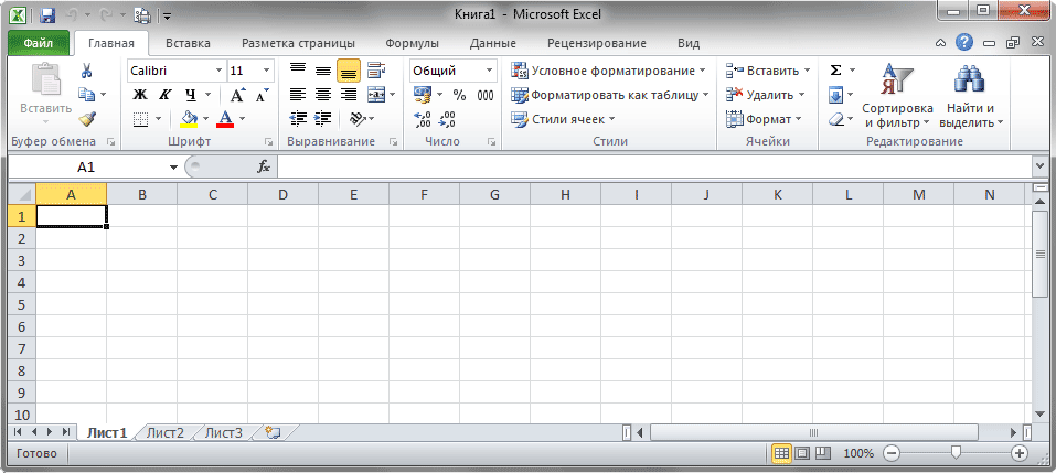
Interface and Management
If you are already familiar with the Word editor, it will not be difficult to understand the Excel interface. After all, it is based on the same Tape, but only with another set of tabs, groups and teams. At the same time, to expand the workspace, some tab groups are displayed on the display only if necessary. You can also roll the tape at all by clicking on the active tab twice the left mouse button or by pressing the Ctrl + F1 key combination. Returning it to the screen is carried out in the same way.
It is worth noting that in Excel for the same command, several ways to call it can be provided immediately: through the tape, from the context menu or using a combination of hot keys. Knowledge and use of the latter can greatly speed up the work in the program.
The context menu is context-sensitive, that is, its content depends on the fact that the user does at the moment. The context menu is called by pressing the right mouse button almost on any object in MS Excel. This saves time, because it displays the most frequently used commands to the selected object.
Despite such a variety of management, the developers went further and provided users in Excel 2010 the ability to make changes to embedded tabs and even create their own with those groups and commands that are used most often. To do this, click right-click on any tab and select item. Setting tape.

In the window that opens, in the menu on the right, select the desired tab and click on the button Create tab or To create a group, and in the left menu, the desired command, then click the button Add. In the same window, you can rename existing tabs and delete them. To cancel erroneous actions there is a button Resetreturning the settings of the tabs to the initial one.
Also most frequently used commands can be added to Fast access panellocated in the upper left corner of the program window.
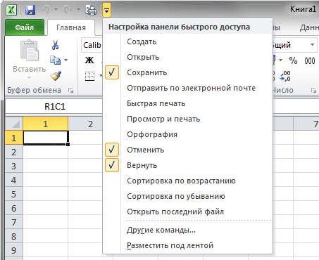
You can make it by clicking on the button. Setting the Quick Access Panelwhere it is enough to choose the desired command from the list, and in the absence of in it necessary, click on the item Other teams.
Entering and editing data
Created by B. Excel files They are called workbooks and have the expansion "XLS" or "XLSX". In turn, the workbook consists of several working sheets. Each work sheet is a separate spreadsheet, which, if necessary, can be interrelated. The active working book is the one with which you currently work, for example, in which enter the data.
After starting the application, a new book is automatically created with the name "Book1". By default, the workbook consists of three working sheets with names from "List1" to "List3".
Working field leaf Excel Divided into many rectangular cells. The horizontal cells make up lines, and vertically - columns. For the ability to study a large amount of data, each work sheet of the program has 1,048,576 lines of numbered numbers and 16,384 columns designated by the letters of the Latin alphabet.
Thus, each cell is a place of intersection of various columns and lines on a sheet forming its own unique address consisting of the letter of the column and the number of the string with which it belongs. For example, the name of the first cell is A1, as it is at the intersection of the column "A" and the lines "1".
If the application is enabled Row of formulaswhich is located immediately under Ribbonthen to the left of it is Field namewhere the name of the current cell is displayed. Here you can always enter the name of the scholar cell, to quickly transition to it. This feature is especially useful in large documents containing thousands of rows and columns.
Also for viewing different areas of the sheet, the scroll strips are located downstairs. In addition to it to move on the working excel area You can use the arrow keys.
![]()
To start entering data into the desired cell, it must be allocated. To go to the desired cell, click on it with the left mouse button, after which it will be surrounded by a black frame, the so-called active cell indicator. Now just start typing on the keyboard, and all the information entered will be provided in the selected cell.
When entering data into the cell, you can also use the formula string. To do this, highlight the desired cage, and then click on the Formula Row field and start printing. At the same time, the information entered will be automatically displayed in the selected cell.
After entering the data entry, press:
- The "Enter" key - the next active cell will be the bottom of the bottom.
- The "Tab" key - the next active cell will be the cell on the right.
- Click on any other cell, and it will become active.
To change or delete the contents of any cell, click on it two times the left mouse button. Move the flashing cursor to the desired place to make the necessary edits. As in many other applications, the arrows, "del" and "backspace" keys are used to delete and making corrections. If desired, all necessary edits can be made in the formula row.
The amount of data that you will be inserted into the cell is not limited to its visible part. That is, the working field cells of the program may contain both one digit and several text paragraphs. Each excel Cell Can accommodate up to 32,767 numeric or text characters.
Formatting data of cells
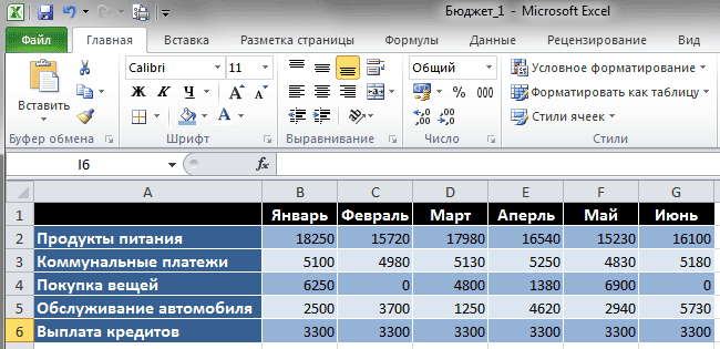
After entering the names of rows and columns we get a table of this type:
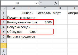
As can be seen from our example, several names of the costs of the costs "came out" beyond the boundaries of the cell and if the neighboring cell (cells) also contain some information, the introduced text partially overlaps to it and becomes invisible. Yes, and the table itself looks quite ugly and non-primable. At the same time, if you print such a document, then the current situation will be saved - to disassemble what it will be quite difficult to make sure that you can make sure of the figure below.

To do tabular document More neat and beautiful, often you have to change the size of rows and columns, the font of the contents of the cell, its background, to align text, add borders and so on.
First, let's put the left column in order. Move the mouse cursor on the border of the columns "A" and "B" in the string where their names are displayed. When changing the mouse cursor to a characteristic symbol with two multidirectional arrows, press and hold the left key, drag the dotted line in the desired direction to expand the column until all the names are appropriate within the same cell.
The same actions can be done with a string. This is one of the easiest ways to change the size of the height and the width of the cells.
If you need to specify the exact dimensions of the rows and columns, then for this on the tab the main in a group Cells Select Format. In the menu that opens using commands String height and Column width You can set these parameters manually.
It is very often necessary to change the parameters in the rod of several cells and even a whole column or string. In order to select a whole column or string, click on its name from above or on its number on the left, respectively.

To highlight the neighboring cells, blaming their cursor, hold the left mouse button. If you need to highlight the scattered table fields, then press and hold the "Ctrl" key, then click the mouse over the necessary cells.
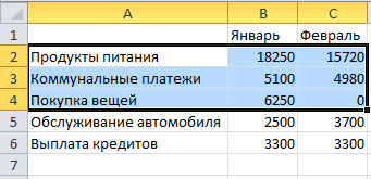
Now that you know how to highlight and format several cells at once, let's align the name of the months in our table in the center. Different content leveling commands inside the cells are on the tab. the main in a group with speaking name Alignment. At the same time, for a table cell, this action can be made both relative to the horizontal direction and vertical.

Circle cells with the name of months in the table header and click on the button Align in the center.
In a group Font On the tab the main You can change the type of font, its size, color and inscription: fat, rush, emphasized and so on. Also, there are buttons for changing the boundaries of the cell and the color of its fill. All these functions will use us for further changes in the appearance of the table.
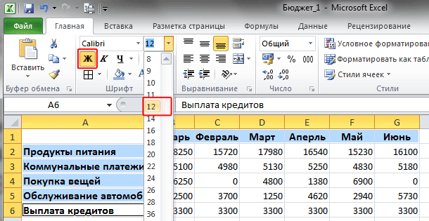
So, for starters, let's increase the font of the names of the columns and columns of our table up to 12 points, as well as make it fat.
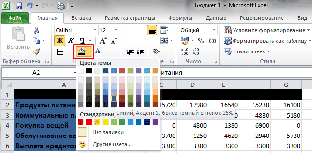
Now we highlight the top line of the table and install it a black background, and then in the left column cells with A2 by A6 - dark blue. You can do this using the button Color fill.
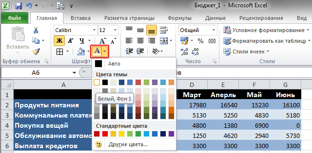
Surely you noticed that the color of the text in the top row merged with the color of the background, and in the left column, the names are read bad. Correct this by changing the color of the font using the button Text color on white.
Also with the help of a familiar team Color fillwe gave the background of even and odd rows with numbers a different blue tint.
So that the cells do not merge, let's define the borders. The definition of boundaries occurs only for the dedicated area of \u200b\u200bthe document, and can be done both for one cell and for the entire table. In our case, select the entire table, then click on the arrow next to the button Other borders All in the same group Font.

In the menu that opens, a list of fast commands is displayed, with which you can select the display of the desired boundaries of the selected area: lower, top, left, right, external, all, etc. Also here contains commands for drawing borders manually. At the bottom of the list there is a paragraph Other borders Allowing more detailed to set the necessary parameters of the boundaries of the cells that we use.
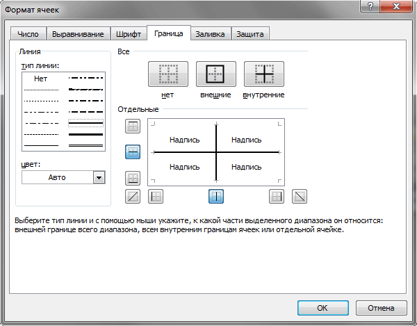
In the window that opens, first select the border line type (in our case, thin solid), then its color (choose white, since the background table is dark) and finally, those borders that will have to be displayed (we chose internal).
As a result, using a set of commands of just one group Fontwe transformed a non-pieces appearance of the table in quite presentable, and now knowing how they work, you can independently invent your unique styles to design spreadsheets.
Cell data format
Now, to complete our table, you must properly arrange the data that we enter there. Recall that in our case it is cash spending.
In each of the cells spreadsheet You can enter different types of data: text, numbers, and even graphic images. That is why in Excel there is a concept as "cell data format", which serves for the correct processing of the information you enter.
Initially, all cells have General formatallowing them to contain both text and digital data. But you have the right to change it and choose: numeric, monetary, financial, interest, fractional, exponential and formats. In addition, there are date formats, postal index time, phone numbers and table numbers.
For the cells of our table containing the names of its rows and columns, the general format is quite suitable (which is set by default), as they contain text data. But for the cells in which budget expenditures are introduced more cash format.
Highlight in the cell table containing information on monthly costs. On the ribbon in the tab the main in a group Number Click on the arrow next to the field Numeric format, After that, the menu will open with the list of the main available formats. You can choose Monetary right here, but we will choose the lowest line for a more complete acquaintance Other numeric formats.
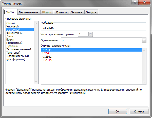
In the window that opens, the name of all numeric formats will be displayed in the left column, including additional, and in the center, various settings for their display.
By selecting a cash format, you can see the window on top, then how the value in the table cells will look like. Slightly below the mono set the number of decimal signs. To kopecks did not clutch the fields of the table, exhibit here a value equal to zero. Next, you can choose a currency and mapping of negative numbers.
Now our tutorial finally accepted the completed view:
By the way, all the manipulations that we have done with the table are higher, that is, the formatting of the cells and their data can be performed using the context menu by right-clicking on the selected area and selecting the item Format cells. In the window that opens for all operations considered by us, there are tabs: Number, Alignment, Font, The border and Fill.
Now at the end of the program, you can save or print the result. All these commands are in the tab. File.
Conclusion
Probably, many of you will look at the question: "Why create a similar kind of table in Excel, when all the same can be done in Word using ready-made patterns?". So it is so, just to produce all sorts of mathematical operations on cells in a text editor is impossible. You have the same information in cells, you almost always put on your own, and the table is only a visual view of the data. Yes, and the volumetric tables in Word are not entirely convenient.
In Excel, the same way is on the contrary, the tables can be as large, and the cell value can be entered both manually and automatically calculate with the help of formulas. That is, here the table acts not only as visual materialBut also as a powerful computational and analytical tool. Moreover, the cells among themselves can be interconnected not only within one table, but also contain values \u200b\u200bobtained from other tables located on different sheets and even in different books.
You will learn how to make the "smart" table in the next part, in which we will get acquainted with the main computational capabilities of Excel, the rules for constructing mathematical formulas, functions and many others.