How to fix the first two columns in Excel. Fastening sheet areas. Formatting cells by condition
Grouping data
When you prepare the catalog of goods with prices, it would be good to worry about the convenience of using it. A large number of positions on one sheet forces to use the search, but what if the user only makes the choice and does not have an idea of \u200b\u200bthe name? In online directories, the problem is solved by the creation of groups of goods. So why and in the book Excel do not do the same?
It is easy to organize a grouping. Select several rows and click Group On the tab Data (See Fig. 1).
Figure 1 - Grouping button
Then specify the grouping type - by strings (See Fig. 2).

Figure 2 - Selecting a grouping type
As a result, we get ... Not what we need. Rows of goods merged into the group specified under them (see Fig. 3). In the catalogs, usually first goes a header, and then the contents.

Figure 3 - Grouping Lines "Down"
This is not a program error. Apparently, the developers considered that the lines group are mainly engaged in financial statements, where the final result is excreted at the end of the block.
To group up the uplinks you need to change one setting. On the tab Data Click on the small arrow in the lower right corner of the section Structure (See Fig. 4).

Figure 4 - Button that is responsible for outputting the structure of the structure settings
In the settings window that opens, uncheck the checkbox from the point Results in lines under the data(see Fig. 5) and click OK.
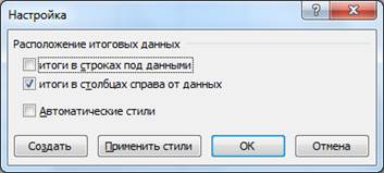
Figure 5 - Structure Settings Window
All the groups you have managed to create will automatically change to the "upper" type. Of course, set parameter will affect the further behavior of the program. However, you will have to shoot this check box for eVERY new leaf and every new Excel book, because The developers did not provide for the "global" installation of the grouping type. Similarly, you can also use different types of groups within one page.
After you have distributed goods by category, you can collect categories in larger sections. A total of nine grouping levels.
Disadvantage When using this feature, it is necessary to press the button. OK In the pop-up window, and collect unrelated ranges for one approach fails.

Figure 6 - Multi-level directory structure in Excel
Now you can open and close part of the directory, click on the pluses and minuses in the left column (see Fig. 6). To deploy the entire level, press one of the numbers at the top.
To bring the strings to a higher level of hierarchy, use the button To ungrade tabs Data. You can completely get rid of the group using the menu item Remove structure (See Fig. 7). Be careful, it is impossible to cancel the action!

Figure 7 - Remove the string grouping
Fastening sheet areas
Often enough when working with excel Tables There is a need to fasten some areas of the sheet. There may be placed, for example, headers of strings / columns, company logo or other information.
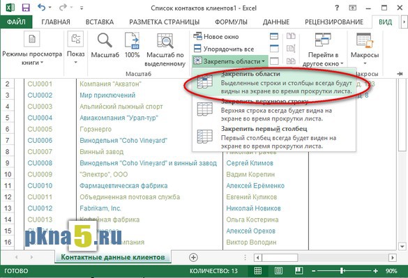
If you fix the first string or first column, then everything is very simple. Open tab View and in the drop-down menu To fix areas Select respectively paragraphs Secure the top row or Secure the first column (See Fig. 8). However, simultaneously and the line, and the column will not be able to "freeze" in this way.
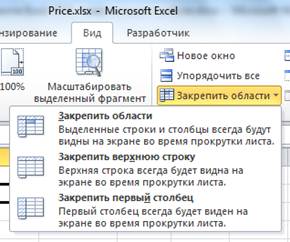
Figure 8 - fix the string or column
To remove the fixation, select the point in the same menu Remove the fixation of the regions (item replaces the string To fix areasIf the page applied "freezing").
But the fixing of several rows or areas from rows and columns is not so transparent. You highlight three lines, click on item To fix areasAnd ... Excel "freezes" only two. Why is that? An even worsede option is possible when the areas are fixed in an unpredictable way (for example, you allocate two lines, and the program puts the border after the fifteenth). But we will not write it up for underwriting developers, because the only correct use of this feature looks different.
You need to climb the mouse in the cell below the lines that you want to fix, and, accordingly, the right of fixed columns, and then choose the item To fix areas. Example: in Figure 9, a cell highlighted B 4.. It means that three lines and the first column will be fixed, which will remain in their places when scrolling the sheet as horizontally, and vertically.

Figure 9 - fix the area from rows and columns
You can apply the background fill for fixed areas to specify the user to the special behavior of these cells.
Turning sheet (replacement of rows on columns and vice versa)
Imagine this situation: you worked for a few hours on a set of tables in Excel and suddenly realized that it was incorrectly designed by the structure - the column headers should be painted on lines or strings on columns (it does not matter). Draw everything manually again? Never! Excel provides a function that allows you to carry out a "rotation" of a sheet by 90 degrees, thus moving the contents of rows in the columns.
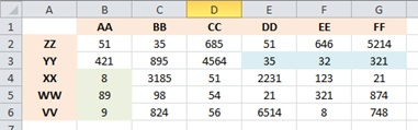
Figure 10 - Source Table
So, we have some table that you need to "rotate" (see Fig. 10).
- Select cells with data. There are precisely cells, not strings and columns, otherwise nothing will work.
- Copy them to the clipboard combination of keys
or in any other way. - Go to an empty sheet or free space of the current sheet. Important note: You can not insert over current data!
- Insert data to the key combination
and in the insert parameter menu select the option Transpose (See Fig. 11). Alternatively, you can use the menu Insert from the tab the main (See Fig. 12).
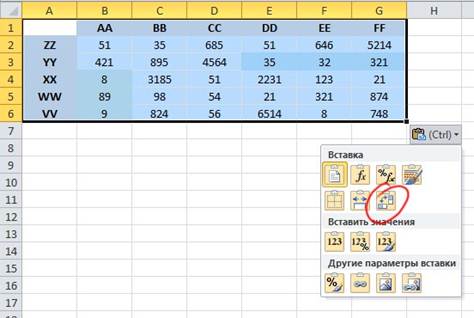
Figure 11 - Insert with transposition
![]()
Figure 12 - Transposition from the main menu
That's all, turning the table is made (see Fig. 13). At the same time, formatting is preserved, and the formulas change in accordance with the new position of the cells - no routine work will be required.
Figure 13 - result after turning
Show formula
Sometimes there is a situation when you cannot find the desired formula among the large number of cells, or just do not know what and where to search. In this case, you can use the ability to display not the result of calculations, but the initial formulas.
Press the button Show formulas On the tab Formulas (See Fig. 14) to change the data view on the sheet (see Fig. 15).

Figure 14 - Button "Show Formulas"

Figure 15 - Now the formula is visible on the sheet, and not the results of the calculation
If you are difficult to navigate to the cell addresses displayed in the formula string, click the button. Influencing cells from the tab Formulas (See Fig. 14). Dependencies will be shown by arrows (see Fig. 16). To use this feature, you must first allocate one Cell.
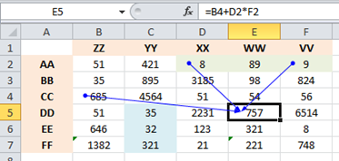
Figure 16 - Cell dependencies are shown by arrows
Hide the dependences by pressing the button Remove arrows.
Transfer lines in cells
Frequently often in Excel's books there are long inscriptions that are not placed in a cell in width (see Fig. 17). You can, of course, push the column, but not always this option is acceptable.
Figure 17 - The inscriptions are not placed in cells.
Select cells with long inscriptions and click Transfer text on the The main thing tab (see Fig. 18) to go to a multi-line display (see Fig. 19).
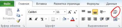
Figure 18 - Text Transfer Button

Figure 19 - Multi-line text display
Turning text in cell
Surely you came across the situation when the text in the cells had to be placed not horizontally, but vertically. For example, to sign a group of strings or narrow columns. In Excel 2010 there are means to rotate text in cells.
Depending on your preferences, you can go in two ways:
- First create an inscription, and then turn it out.
- Configure the turn of the inscription in the cell, and then enter the text.
Options vary slightly, so we consider only one of them. To start, I combined six lines into one using the button Combine and put in the center on the The main thing tab (see Fig. 20) and introduced a generalizing inscription (see Fig. 21).
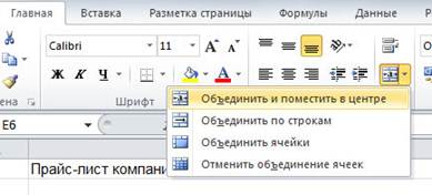
Figure 20 - cell combining button
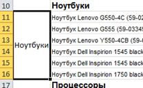
Figure 21 - First create a horizontal signature

Figure 22 - Text Turn Button
You can further reduce the column width (see Fig. 23). Ready!
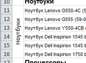
Figure 23 - Vertical Cell Text
If there is such a desire, the angle of rotation of the text you can specify manually. In the same list (see Fig. 22) select item Cell leveling format And in the window that opens, set an arbitrary angle and alignment (see Fig. 24).
Figure 24 - Set an arbitrary angle of text
Formatting cells by condition
Capabilities conditional formatting Appeared in Excel for a long time, but by the 2010 version were significantly improved. Perhaps you will not even have to understand the intricacies of the creation of rules, because Developers have provided many blanks. Let's see how to use conditional formatting in Excel 2010.
The first thing to be done is to highlight cells. Next, by The main thing Tap button Conditional formatting and select one of the blanks (see Fig. 25). The result will be displayed on the sheet right away, so you will not have to go through the options for a long time.
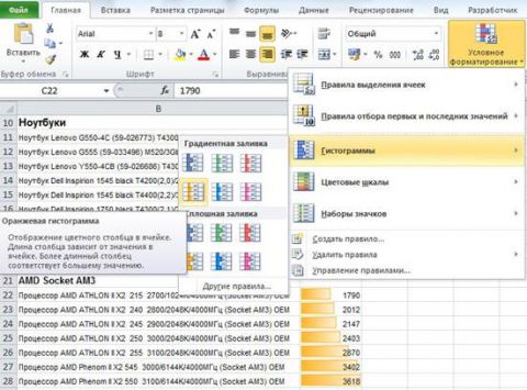
Figure 25 - Select conditional formatting workpiece
Histograms look quite interesting and well reflect the essence of price information - the higher, the longer the segment.
Color scales and icons sets can be used to indicate different states, for example, transitions from critical costs to permissible (see Fig. 26).
Figure 26 - Color scale from red to green with intermediate yellow
You can combine histograms, scales and badges in one cell range. For example, histograms and badges in Figure 27 show the permissible and excessively low performance of devices.
Figure 27 - Histogram and set of icons reflect the performance of some conditional devices
To remove the conditional formatting of the cells, select them and select the Conditional Format menu. Delete rules from selected cells (See Fig. 28).

Figure 28 - We delete the rules of conditional formatting
Excel 2010 uses blanks for quick access to conditional formatting capabilities, because Setting up your own rules for most people is far from obvious. However, if the templates provided by the developers are not satisfied with you, you can create your own rules for the design of cells on various conditions. A complete description of this functional is beyond the framework of the current article.
Using filters
Filters allow you to quickly find the desired information in a large table and represent it in a compact form. For example, from a long list of books, you can choose the works of Gogol, and from the price list of the computer store - Intel processors.
Like most other operations, the filter requires the selection of cells. However, it is not necessary to allocate the entire table with data, it is enough to note the strings above the required data columns. This significantly increases the convenience of using filters.
After the cells are highlighted, on the tab the main Press the button Sorting and filter and select Filter (See Fig. 29).
Figure 29 - Create filters
Now cells will be converted to drop-down lists, where you can specify the sample parameters. For example, we are looking for all mentions about Intel in column Name of product. To do this, choose a text filter Contains (See Fig. 30).
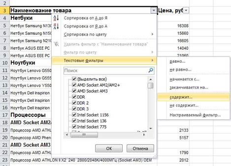
Figure 30 - Create a text filter
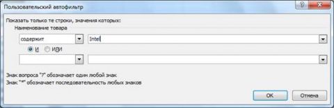
Figure 31 - Create a filter according to the word
However, it is much faster to achieve the same effect by entering the word in the field Search The context menu shown in Figure 30. Why then cause an additional window? It is useful if you want to specify several sampling conditions or select other filtering parameters ( does not contain, starts with ..., ends on ...).
Other parameters are available for numeric data (see Fig. 32). For example, you can choose the 10 largest or 7 smallest values \u200b\u200b(the number is configured).
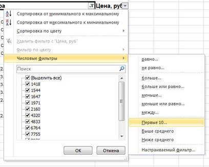
Figure 32 - Numeric filters
Excel filters provide sufficiently rich features comparable to select SELECT query in database management systems (DBMS).
Displays information curves
Information curves (infocrilli) - innovation in Excel 2010. This feature allows you to display the dynamics of changes in the numerical parameters directly in the cell without resorting to the construction of the chart. Changes in numbers will be immediately shown on the micrograph.
Figure 33 - Infoctern Excel 2010
To create an infocal, press one of the buttons in the block. Infocrilli On the tab Insert (See Fig. 34), and then set the range of cells for constructing.
Figure 34 - inserting infocriva
Like diagrams, informational curves have many parameters to configure. More detailed guide On the use of this functional described in the article.
Conclusion
The article addressed some useful features of Excel 2010, accelerating work improving appearance Tables or ease of use. It does not matter whether you create a file yourself or use someone else's - in Excel 2010 there are functions for all users.
22-07-2015In this material, the answer on how to fix the string in Excel. We will see how to fix the first (top) or arbitrary string, and also we will analyze how to fix the area in Excel.
Fastening a string or column in Excel is an extremely useful feature, especially to create lists and tables with a large number of data placed in cells and columns. Signing the string You can easily track the headlines of certain columns, which means save time instead of an infinite scrolling up-down.
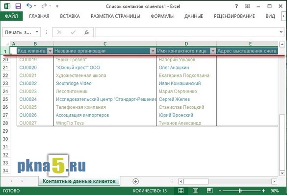
Consider an example. In the figure below, we see the first string that is the headlines of the columns.
Agree, we will inconveniently make and read data from the table, if we do not know or see headers at the top. Therefore, fasten the top period in Excel as follows. In the Excel top menu, we find the item "View", in the opening submenu, choose "consolidate the area", and then select subparagraph "secure the top string".
These simple actions for fixing the string allow you to scroll through the document and at the same time understand the value of the headers of the strings in Excel. I repeat - it is convenient when a large number of lines.
It must be said that the same effect can be achieved if you first select the cells of the entire first line, and then applying the first subparagraph already a well-known submenu "Fasten the Area" - "Secure the Area":
Well, now about how to fix the area in Excel. Initially, highlight the area of \u200b\u200bthe cells of the excel you want to constantly see (secure). It can be several lines and an arbitrary number of cells. As you already probably guess, the path to this functions remains the same: the menu item "View" → Next "Fasten the Area" → Next subparagraph "Secure the Area". On the top figure it is illustrated.
If for some reason you failed to correctly fix the strings or areas in Excel, go to the "View" menu → "Secure the Area" → Select "Remove Consolidate Region". Now you can try again slowly fix the desired lines and the area of \u200b\u200bthe document.
Finally, I will say that the first column is also consolidating. We also act → Menu "View" → "Secure the Area" → Select "Secure the first column".

Good luck to your documents in Excel, do not make mistakes and save your time using additional features and tools of this editor.
We have repeatedly spoke about the tabular editor from Microsoft - about excel program. The entire package of office programs is rightfully is the market leader. And this leadership is fairly easily explained by the presence of a huge functional. Moreover, with each version it is replenished.
In fact, about a tenth of all functions is not used by an ordinary user, so many do not even know about their existence and make it manually what can be done automatically. Or spend time, adapting to certain restrictions and inconveniences. Today we want to tell you how to consolidate the area in Excel. In other words, the program has a function, thanks to which you can consolidate the document cap for your convenience.
Fix the area (header) in Microsoft Excel
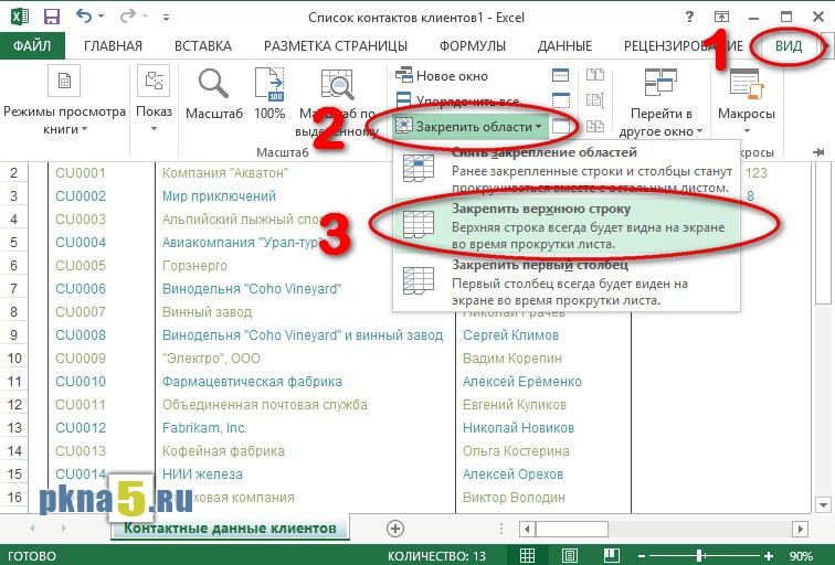
Well, we will not more pull. Let's immediately consider the process of fastening the area you need as a stationary cap, which will always remain from above (or on the side) wherever you scroll through the document. So, you must do the following actions to achieve the desired result:- First of all, go to the "View" tab, then click on the button "Fasten the area";
- Now you must choose the desired fixing option. There are only three of them:
Thus, the choice of a specific item depends solely on your needs.
Fixing and lines, and columns at the same time
Be that as it may, these options are suitable only if you want to highlight one line or one column anywhere in the document. But what to do if you need to fix it immediately and the string, and the column so that they are displayed constantly? Let's figure out:
As you can see, nothing complicated in both cases. This is a matter of literally a few minutes. That is why the MS Office office software package (in their number includes Excel) is really the most popular software for editing all types of text and graphic data: any action can be automated or simplified as much as possible, the main thing is to remember how it all is done.
This manual is relevant not only for Excel 2013, on which it has been demonstrated, but also for older - the difference may be in the location of the elements, no more. Therefore, if you have another version, do not be lazy to make a couple of unnecessary movements with the mouse.