Given a fragment of a spreadsheet after performing calculations
Interactive trainer 7 exam DEMO 2017
Spreadsheets. Representing data in spreadsheets
If you have any questions, doubts or comments, write ...
Analysis of the solution to task 7.1 of the USE 2016 demo
Spreadsheets.
7.1 Given a fragment spreadsheet... The formula was copied from cell E4 to cell D3. When copying, the addresses of the cells in the formula were automatically changed. What became the numeric value of cell D3:
Note: the $ sign denotes absolute addressing.
Decision:
Recall that absolute addressing does not change the value of the formula when moving to another cell, unlike relative. We use this knowledge as follows.
The formula is in cell E4, and its first team $ B2
literally means this:
In any cell, no matter where we put the formula, we take the value that lies strictly in column B (since B is in front of $), but two lines higher than where we stand ..
why exactly higher and 2? We just stand in line number 4, but we need to take it from the second (after B is 2), which means that we need to go up 2 lines.
The sign to multiply speaks for itself. And the second command can be translated as follows:
Consider the second part of the formula From $ 3
and write down what this means in simple language:
In any cell, no matter where we put the formula, we take the value that lies two columns to the left of the new place, but strictly in the third row.
Why exactly two columns to the left? From cell E4 to C, how many columns you need to go through - two, here are two steps to the left and remember. Why exactly from the third line? Only because there is a $ sign before the triplet, which tells us that the triplet does not change when transferred.
It remains to stand in the specified cell and repeat the rules formed in cell E2.
So, we stand in cell D 3 and multiply the values \u200b\u200bobtained by the "red" and "blue" commands.
OfD 3 we take the value that lies strictly in column B and two lines higher from the place where we stand, that is, the value of cell B1
OfD3 we take the value that is two columns to the left and necessarily from the third row, i.e. cell valueB3
It remains to multiply these values \u200b\u200bB1 * B3 \u003d 4 * 2 \u003d 8.
Interactive trainer 7.1 demo USE 2016
Presentation of data in spreadsheets in the form of charts and graphs.
Analysis of the solution to task 7.2 of the USE demo 2016
Presentation of data in spreadsheets in the form of charts and graphs.
7.2 Given a fragment of a spreadsheet:
??? |
6 |
10 |
|
\u003d (A1–3) / (B1–1) |
\u003d (A1–3) / (C1–5) |
\u003d C1 / (A1–3) |
What integer number must be written in cell A1 so that the diagram constructed after performing the calculations by the values \u200b\u200bof the range of cells A2: C2 corresponds to the figure? It is known that all values \u200b\u200bof the range over which the chart is plotted have the same sign.
From the figure it follows that as a result of the calculations, two identical numbers should be obtained, and the third is equal to their sum or twice as much of them. It is easy to guess that the values \u200b\u200bof the first and second formulas are equal, since they have the same numerators and denominators. B1-1 \u003d 5 and C1-5 \u003d 5.
Therefore, we can write (A1–3) / (B1–1) \u003d (A1–3) / (C1–5) whence it follows that
2 * (A1-3) / 5 \u003d 10 / (A1-3)
2X-6 \u003d 50 / (x-3)
2 (x-3) (x-3) \u003d 50
(x-3) (x-3) \u003d 25
X-3 \u003d 5
So the correct answer is 8
Interactive trainer 7.2 demo version of the exam 2016
Presentation of data in spreadsheets in the form of charts and graphs.
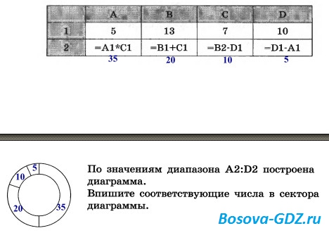
2. Given a fragment of a spreadsheet in the formulas display mode. 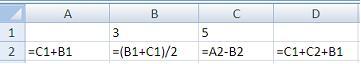 After performing the calculations, a chart was built using the values \u200b\u200bof the cell range A2: D2. Indicate the resulting diagram.
|
|

3. The correct record of the formula for MS Excel spreadsheets among those given is ...
|
A1 / 3 + S3 * 1.3E – 3 |
|||
|
A1 / 3 + S31,3E – 3 |
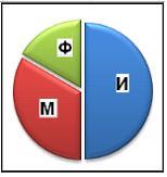
4. The table shows data on the number of winners of the Olympiad in informatics (I), mathematics (M) and physics (F) in three cities of Russia: 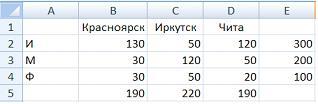 Column E counts the number of winners for each city, and row 5 - the number of winners for each subject. Diagram
 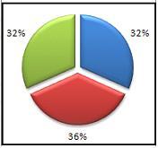 built on ...
5. A fragment of a spreadsheet is given. For this fragment of the table, it is true that the cell ... 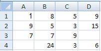
6. Automate the operation of entering in related tables allows ... 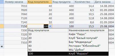
8. Given a fragment of a spreadsheet: 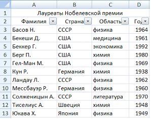 The number of records that match the next custom autofilter conditions
 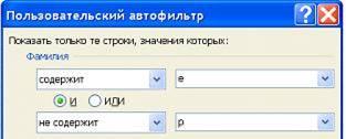 equal ...
9. Given a fragment of a spreadsheet.  ... The number of records that match the autofilter condition
  equal ...
10. A fragment of a spreadsheet in the formulas display mode looks like: 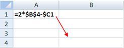 Formula from cell A1copied to cell B3... In a cell B3the formula appears ...
|
2 * $ B $ 4 - $ C3 |
|||
|
4 * $ B $ 6 - $ C3 |
|||
|
2 * $ C $ 4 - $ D1 |
|||
|
2 * $ C $ 6 - $ D3 |
11. Given a fragment of a spreadsheet 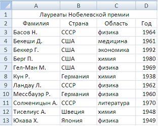
 information about L. Landau will begin with cell ...
12. Given a fragment of a spreadsheet  ... The number of records that match the advanced filter conditions
 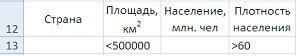 equal ...
13. Given a fragment of a spreadsheet in the formulas display mode. 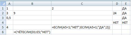 After performing the calculations ...
14. When you copy the contents of cell A2 to cells B2 and A3, formulas appeared in them. 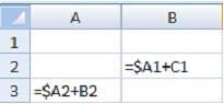 Cell A2 contains the formula ...
15. Given a fragment of a spreadsheet ... After sorting by conditions  in cell A9 there will be a surname ...
|
Landau L. |
||
|
Becker G. |
||
|
Bekesy D. |
16.
The diagram shows the number of winners of the Olympiad in informatics (I), mathematics (M) and physics (F) in three cities of Russia:  The diagram that correctly reflects the ratio of winners from all cities in each subject is ...
|
|
17. Given a fragment of a spreadsheet in the formulas display mode:  After performing calculations, the value in the cell C6will equal ...
18. In cell A1, the numeric constant is written in exponential format. ![]() In numerical format, it will be written as ...
In numerical format, it will be written as ...
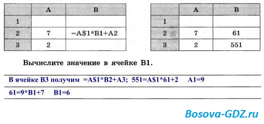
19. Given a fragment of a spreadsheet in the formulas display mode: ![]() Formula from cell B2was copied into a cell B3... After that, a fragment of the spreadsheet in the display mode of values \u200b\u200btook the form:
Formula from cell B2was copied into a cell B3... After that, a fragment of the spreadsheet in the display mode of values \u200b\u200btook the form: 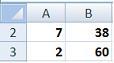 Cell value B1equal ...
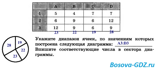
20. A fragment of a spreadsheet and a diagram are given. The range of cells, according to the values \u200b\u200bof which the chart was built, is ... 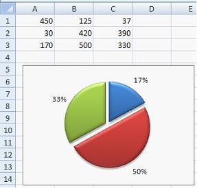
21. The teleconference is attended by teachers of mathematics, physics and computer science. Teachers have different qualifications: no category (BC), II, I, or the highest (VC) category. Diagram 1 shows the number of teachers with different skill levels, while Diagram 2 shows the distribution of teachers by subject. Diagram 1 Diagram 2 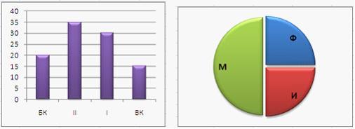 From the analysis of both diagrams, it follows that all teachers ...
|
informatics can have the highest category |
|||
|
mathematicians can have II category |
209. A fragment of a spreadsheet is given in the formulas display mode. What is the result of the calculations in cell C3?
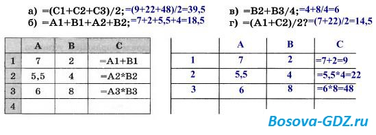
210. Fragment of a spreadsheet contains numbers and formulas. What value will be in cell C4 if it contains the formula:
211. One of the cells in the spreadsheet contains a formula. Write down the arithmetic expression corresponding to it:

212. Specify the number of cells in the ranges:

213. Fragment of a spreadsheet contains numbers and formulas. Write down the values \u200b\u200bin the cells of the ranges C2: C3, D2: D3, E2: E3, F2: F3, if they copied the formulas of their cells C1, D1, E1, F1, respectively.

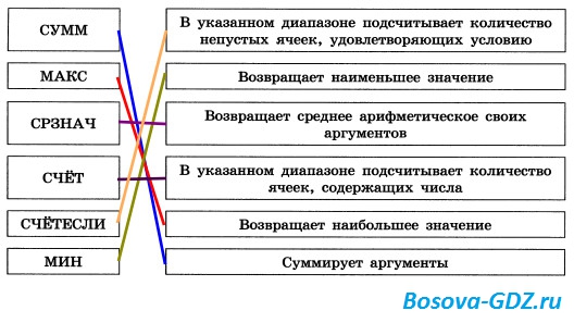
214. Establish a correspondence between the names of the functions and the resulting actions.
215. Fragment of a spreadsheet contains numbers. What value will be in cell C4 if it contains the formula:

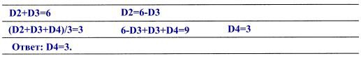
216. In the spreadsheet, the formula value \u003d SUM (D2: D3) is 6, and the formula value \u003d AVERAGE (D2: D4) is 3. What is the value in cell D4?
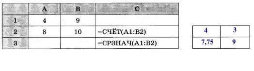
217. Fragment of a spreadsheet contains numbers and formulas. Determine the values \u200b\u200bin cells C2 and C3. What will these values \u200b\u200bbe if you delete the value in cell A1?
218. Given a fragment of a spreadsheet in the formulas display mode. Write down the values \u200b\u200bin the cells of the ranges C2: C3, D2: D3, if they copied the formulas from cells C1, D1, respectively.
219. Given a fragment of a spreadsheet in the formulas display mode. After the contents of cell B2 were copied into cell B3, a fragment of the table in the results display mode began to look like this:
220. Write a conditional function corresponding to the block diagram:

221. Given a fragment of a spreadsheet in the formulas display mode. Enter in the cells of the range B2: B9 the values \u200b\u200bthat will appear in the spreadsheet after copying the formula from cell B1 to B2: B7.

222. The results of the regional programming competition were entered into a spreadsheet.

223. A fragment of a spreadsheet is given.
224. A fragment of a spreadsheet is given.
225. A fragment of a spreadsheet is given. A chart is built based on the values \u200b\u200bof the range of cells B1: B4.
2. What are the main types of links.
There are two main types of links:1) relative - depending on the position of the formula
2) absolute - position-independent formulas
3. Describe the relative type of links.
A relative reference determines the location of the data cell relative to the cell in which the formula is written, and when the position of the cell containing the formula is changed, the reference changes.4. From the spreadsheet, determine the value in cell C1.
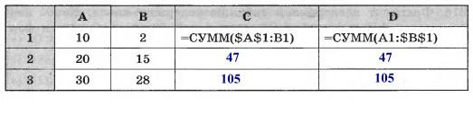
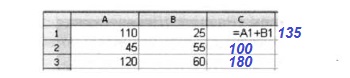
5. A fragment of a spreadsheet is given. Determine the values \u200b\u200bin cells C2 and C3 after copying the formula from cell C1 to them.
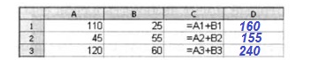
6. A fragment of a spreadsheet is given. Determine the values \u200b\u200bin the cells of the range D1: D3 after copying the formula from cell C3 to them.
7. Describe the absolute type of links.
An absolute reference in a total formula refers to a cell at a specific (fixed) location. In an absolute reference, a $ sign is placed before each letter and number (for example: 2)8. Given a fragment of a spreadsheet. Determine the values \u200b\u200bin cells C2 and C3 after copying the formula from cell C1 to them.
