Introducing formulas to excel. The alignment of the contents of Excel cells. An example of solving a complex formula

Finally, we come to the implementation of one of the features of the "Excel" program - work with formulas for calculations. Cell "D4" should contain the result of multiplying the price of the product in USD. (cell "C4") and today's course (cell "D1"). How to do it? By clicking the left mouse button, mark the cell where the result should be.

To create a formula, left-click on the arrow next to the "AutoSum" button on the toolbar and select "Other functions ...". Or go to the "Insert" menu and select the "Function" item.

A window opens to help you enter the formula. From the list "Category" select the item "Mathematical". (Please note that in fact the program is able to work with various categories of functions. These are financial, and statistical, and work with data, and much more). Find "PRODUCT" in the list of functions. After that, click on the "OK" button.

First, we are asked to indicate the cell from which the data for the first multiplier should be taken. We enter the designation of the desired cell - "C4".

Next step: cell where the second factor is located - "D1". Of course, a specific number can also be used as data, which we enter directly into the field. On the right, we control the result. After entering the data, click on the "OK" button.

In cell "D4" we see the finished result. Now, as soon as we change the data of the course of the conventional unit, the program will make the recalculation itself. Conveniently? Of course!

3 principles of work in Excel

3.1 Working with formulas

Formula- special tool Excel, designed for calculations and data analysis. The formula begins with an "\u003d" sign, followed by the operands and operators. The simplest example of creating a formula can be presented as follows: first, the "\u003d" sign is entered into a cell, then a certain number, after that an arithmetic sign (+, -, * or /), etc. The process of entering the formula is completed by pressing the Enter key - as a result, the result of calculating the formula will be displayed in the cell. Selecting this cell displays the entered formula in the formula bar. However, this way of creating formulas is not always acceptable. This is due to the fact that often for calculations it is necessary to use not just specific numerical values, but the data located in certain cells. In this case, the formula indicates the addresses of the corresponding cells. Any previously created formula can be edited if necessary. To do this, select the appropriate cell and enter the required changes in the formula bar, then press the Enter key. You can also change the formula in the cell itself: to switch to edit mode, you need to place the cursor on it and press the F2 key. Possibilities of the program provide for entering the formula simultaneously into several cells. To do this, select the required range, then enter the required formula in the first cell and press the Ctrl + Enter key combination. The formula can be copied to the clipboard and pasted anywhere on the worksheet. In this case, all used references (cell addresses) in the source formula will be automatically replaced in the receiving formula with similar references corresponding to the new placement of the formula. For example, if you enter the formula \u003d B2 + C1 into cell A1, then copy it to the clipboard and paste it into cell A2, then the formula will look like this: \u003d B2 + C2. If it is necessary not to copy, but to move the formula from one cell to another, select this cell, move the mouse pointer to any of its borders so that it turns into a cross, press the left mouse button and, while holding it, drag the formula to the required place. If you need to copy to the clipboard and then paste into the required place not a formula, but only the value obtained as a result of its calculation, you should select the cell, then copy its contents to the clipboard, move the cursor to the place where you want to paste the data, and select in context menu item Paste special... As a result, a window of the same name will open, in which you should set the switch Paste into position meaning and press OK... In this window, you can select other modes for pasting the contents of the clipboard. Sometimes it is necessary to quickly look through all the formulas in the cells of the worksheet. To do this, run the command Service Options, in the opened window Options in the tab View check the box formulas and press the button OK... As a result, in the cells containing formulas, the formulas themselves will be displayed, and not the result of their calculation. To return to the original display mode, clear this checkbox. To delete a formula, just select the corresponding cell and press the Delete key. If the formula is erased by mistake, then immediately after deleting it, you can restore it to its original place by pressing the Ctrl + Z key combination.

3.2 Working with functions

A function is a formula originally created and embedded in the program, which allows you to perform calculations by specified values \u200b\u200band in a specific order. Each function includes the following constituent elements: "\u003d" sign, name (SUM, AVERAGE, COUNT, MAX, etc.) and arguments. The arguments used depend on the specific function. The arguments can be numbers, links, formulas, text, logical values, etc. Each function has its own syntax, which must be followed. Even a slight deviation from the syntax will lead to erroneous calculations or even to the impossibility of calculation. Functions can be entered either manually or automatically. For automatic input, the function wizard, called with the command Insert Function... You can type the function manually in the formula bar (you must first select the cell into which the data is entered) in the following order: first, the equal sign is indicated, then the name of the function, and then the list of arguments, which are enclosed in parentheses and separated by a semicolon. For example, you need to find the sum of the numbers in cells A1, B2, C5. To do this, enter the following expression in the formula bar: \u003d SUM (A1; B2; C5). In this case, the name is entered in Russian letters, and the arguments, which are cell addresses, are in Latin. After pressing the Enter key, the result of the calculation will be displayed in the active cell. Any function can be used as an argument to any other function. This is called function nesting. The program features include up to seven levels of nesting of functions.

3.3 Working with diagrams

One of the most useful features excel programs is a mechanism for working with diagrams. In general, a chart is a visual graphical representation of available data. The construction of the diagram is carried out on the basis of the information on the worksheet. At the same time, it can be located both on the same sheet with the data on the basis of which it is built (such a diagram is called embedded), or on a separate sheet (in this case, a diagram sheet is created). The chart is inextricably linked to the original data, and whenever it changes, it automatically updates accordingly. To switch to the chart building mode, use the main menu command Insert Diagram... When it is executed, the diagram wizard window opens:
Before using this command, it is recommended to select a range with data on the basis of which the chart will be built. But this range can be specified (or edited) and later, in the second step of building the diagram. The first step in building a diagram is to select its type. The program's capabilities provide for the construction of a wide variety of charts: histograms, graphs, pie, dot, radar, bubble, etc. In the tab Standard a list of standard charts is provided. If none of them meet the user's requirements, you can select a custom chart by clicking the tab Non-standard... To select the required diagram, you need to select its type on the left side of any of the tabs, and the presentation option on the right. If, when executing the command Insert Diagramthe range of data on the basis of which the diagram should be built was selected, then in the diagram wizard window using the button View result you can see how the diagram will look with the currently set settings. The completed chart is displayed on the right side of the tab only when this button is pressed. To go to the second stage of building the diagram, click the button Further... You can end the chart creation process at any time by clicking the Finish button. As a result, a diagram will be created that corresponds to the specified settings. If before executing the command Insert Diagram the data range was not specified, then in the second step in the field Range it should be indicated. Here, if necessary, you can edit the previously specified data range. By switch Ranksthe required option for constructing data series is selected: by rows or by columns of the selected range. In the tab Row you can add and remove data series from a chart. To add a row, click the button Add toand in the box on the right The values specify the range of data that will be used when building the chart. To remove a row from the list, select its name and press the button Delete... In this case, you must be careful, since the program does not prompt you to confirm the delete operation. At the push of a button Further the transition to the third stage of building the diagram is carried out. The window that appears consists of the following tabs: Headings (opens by default) Axles, Grid lines, Legend, Data signatures and Data table... The number of tabs in the window depends on the selected chart type. In the tab Headings in the corresponding fields, the name of the diagram and its axes are entered from the keyboard. The typed values \u200b\u200bare immediately displayed in the display area on the right. The fields on this tab are optional. In the tab Axles the presence of axes (horizontal and vertical) in the diagram is configured. If the display of an axis is disabled, then the axis itself and the values \u200b\u200blocated on it will be absent from the diagram. To enable the display of axes, the X-axis (categories) and Y-axis (values) check boxes must be selected. They are installed by default. To configure the grid lines of the chart, use the tab Grid lines... Here, for each axis, by checking the corresponding boxes, you can enable the display of the main and intermediate lines. In the tab Legend you can control the display of the chart legend. A legend is a list of chart series with an indication of the color of each series. To enable display of the legend, you need to select the checkbox Add legend (it is installed by default). The switch becomes available. Accommodation, which indicates the location of the legend in relation to the diagram: bottom, top right corner, top, right and left. In the tab Data signatures the chart labels are configured. For example, when checking the box meaning the diagram will show the initial data on the basis of which it was built. If you check the box row names,then its name will be displayed above each series of data (the names of the series are displayed in accordance with the list of series that was formed in the second step of building the diagram on the tab Row). If the tab Data table check the box of the same name, then a table with the initial data on the basis of which the diagram is built will be displayed immediately below the diagram. When the button is pressed Further the transition to the fourth, final stage of building the diagram is performed.


At this step, the location of the diagram is determined. If the switch is in position a separate, then after pressing the button Done a separate worksheet will be automatically generated for the chart. By default, this sheet will be named Diagram 1however you can change it if necessary. The process of building the diagram is completed by pressing the button Done... If the switch is set to position available, then in the drop-down list located on the right, select a worksheet from those available in the current book, on which the diagram will be placed. Similarly, you can build a wide variety of diagrams, depending on the needs of the user. To quickly navigate to the data on the basis of which the chart was built, you need to right-click on it and select the item Initial data... As a result, the diagram wizard window will open in the second step, in the field Range which will indicate the boundaries of the range with the original data. In addition, after executing this command, a range with the original values \u200b\u200bwill be selected on the worksheet. If necessary, you can change the location of the diagram at any time. To do this, right-click on it and select Placement in the context menu that opens. This will bring up a dialog box (step 4) in which you can specify a new order for placing the diagram. To remove a diagram from the worksheet, select it by clicking the mouse button and press the Delete key. If you need to delete a chart located on a separate sheet, then you should right-click on the chart sheet shortcut and select the command Delete... In this case, the program will issue an additional request to confirm the delete operation.

3.3.1. Change the appearance of a 3-D chart

E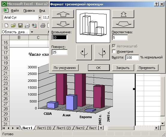

if you are not satisfied appearance of the resulting 3-D chart, some of its parameters can be easily changed. To do this, select the chart and use the command Diagram Volumetric view - the 3D projection format window will open, where you can make changes. When choosing new parameter values, you should pay attention to the button Apply, with which you can see changes in the diagram without closing the editing window. You can also change the elevation and rotation angle of the diagram using the mouse by clicking it in one of the diagram corners and dragging any of the selected corners as needed. It is more convenient to carry out this process while holding down the Ctrl key to make the inner contours of the diagram visible.

3.4 Inserting, editing and deleting notes

The program implements the ability to add a required text comment to any cell - a note. The meaning of this operation is that a note can be displayed either permanently or only when the mouse pointer is placed over the corresponding cell. You can control the display of notes in the window Options in the tab View by switch Notes.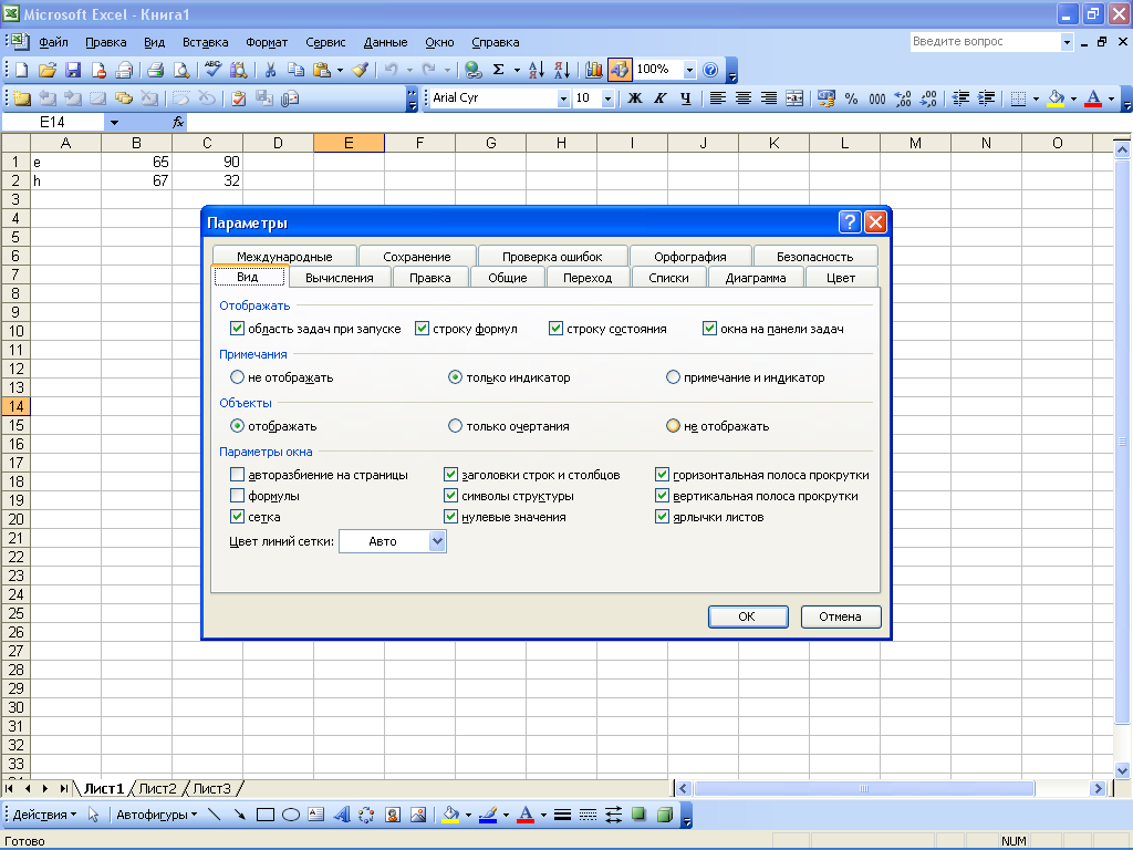

Example note

To add a note to a cell, you need to right-click on it and in the context menu that opens, select Add note... You can also place the cursor in a cell and use the main menu command Insert Note... This will open a note window, which will display the user's name by default. The text of the note can be absolutely arbitrary; it is typed from the keyboard. To complete the entry of a note, simply click anywhere on the worksheet. A previously created note can be edited at any time. To do this, right-click on the cell with the comment and select the Edit Comment command from the context menu. As a result, a note window will open in which you can make the required changes. When you are finished editing, you need to click anywhere on the sheet to make the annotation window disappear. To delete a note, right-click on the corresponding cell and in the opened context menu execute the command Delete note... However, you should be careful, because the program does not issue an additional request to confirm the delete operation. If necessary, you can select all cells of the current worksheet that have notes - to do this, press the key combination Ctrl + Shift + O. To remove notes from all cells on a sheet, select them using the Ctrl + Shift + O combination, then right-click on any of these cells and select the item Delete note.

3.5 Using AutoShapes

Sometimes, in the process of work, it becomes necessary to add graphic objects to the document, designed to highlight a certain fragment of the worksheet, create a diagram or callout, indicate something with an arrow, etc. To facilitate this work, the program implements the ability to use autoshapes. Its essence lies in the fact that the user selects the required shape from the proposed list and then with the mouse pointer indicates the boundaries within which it should be placed. You can access the AutoShapes available in Excel using the toolbar Drawing... To enable its display, you need to run the command View Toolbars Drawing... By default, this panel is located at the bottom of the program window. To work with autoshapes on the toolbar Drawing designed button Autoshapes... When pressed, this menu opens: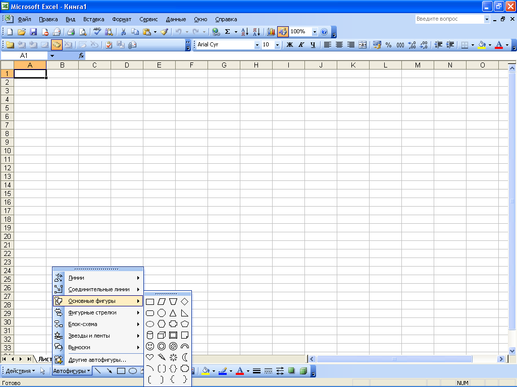


This menu provides access to the autoshapes available in the program. All autoshapes are grouped into thematic submenu groups: Lines, Connectors, Basic Shapes, Curly Arrows, Flowchart, Stars and Ribbons, Leaders, Other Autoshapes. To insert an autoshape into a document, you need to select it in the corresponding submenu, then move the mouse pointer to the place of the worksheet where the autoshape should be inserted and click the mouse button. If necessary, you can stretch the AutoShape to any size the user needs. To do this, after selecting an autoshape, press the mouse button and, while holding it, move the pointer in the required direction. If necessary, using the tools of the Drawing panel, you can additionally decorate the AutoShape (for example, paint the object and its outline with different colors, change the line thickness and type). Any number of autoshapes of arbitrary size can be inserted into any document, depending on the user's needs.

3.6 Setting up and using a data entry form

When working with large amounts of information, it may be necessary to fill in the most different tables significant sizes. To quickly fill in large tables, it is recommended to use the data entry form, which the user customizes independently, depending on the current task. Suppose we want to populate a table with three columns called Profit, Losses and Taxes. This table is located starting at cell A1. First, type the names of the table columns. In our case, in cell A1, enter the value of Profit, in cell B1 - Losses, in cell C1 - Taxes. Then you need to select these cells and run the command Data The form - as a result, this message will appear:


In this window, click the OK button. This will open the data entry form:


The figure shows that the fields located on the left side of this window are named according to the names of the columns of the filled table. The procedure for entering data is as follows: the required values \u200b\u200bare entered in the Profit, Losses and Tax fields, after which the button is pressed Add to... As a result, the first row of the table will be filled in, and the fields are cleared to enter data for the next row, etc. If you need to return to the value entered in the table earlier, use the button Back to... To go to the next values, use the button Further.After all the necessary data have been entered into the table, press the button Close... Similarly, you can fill in any tables, the volume of which is limited only by the size of the worksheet.

3.7 Drawing tables

As you know, the worker excel sheet is a table consisting of cells, each of which is located at the intersection of a row and a column. However, in most cases, you need to arrange a visual representation of a specific table (or several tables) on a worksheet. In particular, you need to assign clear names to the rows and columns that briefly reflect their essence, define the boundaries of the table, etc. To create such tables, a special mechanism is implemented in the program, for access to which the toolbar is intended Border... IN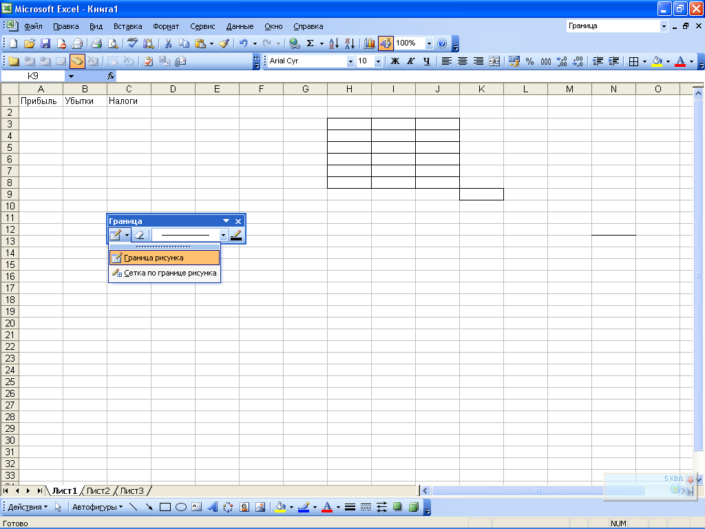

first of all, you should decide on what boundaries you want to draw. For example, you can make the overall border of the table thick and the grid of the table regular. To create a common border, you need to click the button located on the left on the toolbar, and in the menu that opens: select the item Picture border... Then, with the mouse button pressed, the pointer (which will take the form of a pencil) draws the border of the table. In order for each cell to be separated from one another by a border, in the menu of the first button of the Border panel, select the item Boundary gridand then also outline the required range. The type and thickness of the border line is selected in the drop-down list. Here you can find the following line types: dotted, dash-dotted, double, etc. TO

each border line can be assigned a different color if necessary. To select a color, click the button on the right of the toolbar Line color (the name of this button is displayed as a tooltip when you move the mouse pointer over it) and in the menu that opens, select suitable color... The sample of the selected color will be displayed on this button. It should be noted that the borders of the table are not deleted according to the usual rules, that is, using the Delete key. To remove the border, you need on the toolbar Borderpush the button Erase the border, then perform the same actions as when drawing a table (that is, while holding down the mouse button, you need to specify the lines to be erased). To delete a line within one cell, it is enough to bring the pointer to this line, which after pressing the button Erase grthe anitsu will take the form of an eraser and click.

3.8 Calculation of subtotals

When working with tables, it is often necessary to summarize intermediate results (for example, in a table with data for a year, it is advisable to calculate quarterly intermediate results). This can be done, for example, using the standard formula mechanism. However, this option may turn out to be quite cumbersome and not entirely convenient, because for this you need to perform a number of actions: insert new rows (columns) into the table, write the necessary formulas, etc. Therefore, to calculate subtotals, it is advisable to use a specially designed mechanism that is implemented in Excel. In order for the calculation of subtotals using this mechanism to be possible, the following conditions must be met: the first row of the table must contain the names of the columns, and the remaining rows must contain the same type of data. In addition, the table must not have empty rows and columns. First of all, you need to select the table with which you have to work. Then you should go to the mode of setting subtotals - this is done by the command of the main menu Data Results.When it is executed, a dialog box opens. Subtotals.


This window defines the values \u200b\u200bof the parameters listed below.

With every change in - from this drop-down list (it includes the names of all table columns), you need to select the name of the table column, based on the data of which it will be concluded that it is necessary to add a row of subtotals. To understand how the value of this field is processed, consider an example. Suppose the desired column is called Name of product, the first three positions in it are occupied by the product Trousers, the next four - Shoes and two more - T-shirts (all items of the same type differ only in price). If in the calculation window in the field With every change in select value Name of product, then rows will be added to the table with the summary data separately for all trousers, shoes and T-shirts. Operation– here, from the drop-down list, you select the type of operation that should be applied to calculate subtotals. For example, you can calculate the sum, product, display the arithmetic mean, find the minimum or maximum value, etc. Add totals by - in this field, by setting the appropriate checkboxes, you should define the table columns for which the subtotals should be calculated. For example, if in our example the composition of the table in addition to the column Name of productincludes more columns amount and Price (the names of these checkboxes are similar to the names of the table columns), since the calculation of intermediate (and general) totals for a column Name of productmakes no sense . Replace current totals- this checkbox should be checked if it is necessary to replace existing subtotals with new ones. By default, this check box is selected. End of page between groups- if checked, a page break will be automatically inserted after each line of subtotals. By default, this check box is cleared. Totals under data- if this box is checked, then the total lines will be located under the corresponding groups of positions, and if unchecked, then above them. By default, this checkbox is selected! Remove all- when this button is pressed, all existing rows with subtotals will be deleted from the table with the simultaneous closing of the window Subtotals.

At the push of a button OK the process of setting up the calculation of subtotals is completed. Button Cancellation is intended to exit this mode without performing a calculation.

- Formula input order

- Relative, absolute and mixed links

- Using text in formulas

Now let's move on to the fun part - creating formulas. Actually, this is what spreadsheets were designed for.

Formula Entry Procedure

You must enter the formula with the equal sign... This is necessary so that Excel understands that it is the formula that is entered into the cell, and not the data.

Select an arbitrary cell, for example A1. In the formula bar, enter =2+3 and press Enter. The result (5) appears in the cell. And the formula itself will remain in the formula bar.

Experiment with different arithmetic operators: addition (+), subtraction (-), multiplication (*), division (/). To use them correctly, you must clearly understand their priority.

Expressions within parentheses are executed first.

Multiplication and division take precedence over addition and subtraction.

Operators with the same priority are executed from left to right.

My advice to you is to USE BRACKETS. In this case, you will protect yourself from an accidental error in calculations on the one hand, and on the other hand, parentheses make it much easier to read and analyze formulas. If the number of closing and opening parentheses in the formula does not match, Excel will display an error message and suggest an option to fix it. Immediately after entering the closing parenthesis, Excel displays the last pair of parentheses in bold (or some other color), which is very convenient when there are many parentheses in the formula.

Now let's let's try to workusing references to other cells in formulas.

Enter the number 10 in cell A1 and the number 15 in cell A2. In cell A3, enter the formula \u003d A1 + A2. The sum of cells A1 and A2 will appear in cell A3 - 25. Change the values \u200b\u200bof cells A1 and A2 (but not A3!). After changing the values \u200b\u200bin cells A1 and A2, the value of cell A3 is automatically recalculated (according to the formula).

In order not to make mistakes when entering cell addresses, you can use the mouse when entering links. In our case, you need to do the following:

Select cell A3 and enter an equal sign in the formula bar.

Click cell A1 and enter the plus sign.

Click on cell A2 and press Enter.

The result will be the same.

Relative, absolute and mixed links

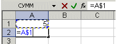
To better understand the link differences, let's experiment.

A1 - 20 B1 - 200

A2 - 30 B2 - 300

In cell A3, enter the formula \u003d A1 + A2 and press Enter.

Now place the cursor on the lower right corner of cell A3, press the right mouse button and drag to cell B3 and release the mouse button. A context menu will appear in which you need to select "Copy cells".

After that, the value of the formula from cell A3 will be copied to cell B3. Activate cell B3 and see what formula turned out - B1 + B2. Why did it happen? When we wrote down the formula A1 + A2 in cell A3, Excel interpreted this record as follows: "Take the values \u200b\u200bfrom the cell located in the current column two rows higher and add with the value of the cell located in the current column one row higher." Those. by copying the formula from cell A3, for example, into cell C43, we get - C41 + C42. This is the beauty of relative links, the formula itself adjusts itself to our tasks.

Enter the following values \u200b\u200bin the cells:

A1 - 20 B1 - 200

A2 - 30 B2 - 300

Enter the number 5 in cell C1.

In cell A3, enter the following formula \u003d A1 + A2 + $ C $ 1. Copy the formula from A3 to B3 in the same way. See what happened. Relative links "adjusted" to the new values, but absolute links remained unchanged.

Try experimenting with mixed links yourself and see how they work. You can refer to other sheets in the same workbook exactly as you would to cells in the current sheet. You can even refer to the sheets of other books. In this case, the link will be referred to as an external link.

For example, to write in cell A1 (Sheet 1) a link to cell A5 (Sheet2), you need to do the following:

Select cell A1 and enter an equal sign;

Click on the "Sheet 2" tab;

Click on cell A5 and press enter;

after that, Sheet 1 will be activated again and the following formula will appear in cell A1 \u003d Sheet2! A5.

Editing formulas is similar to editing text values \u200b\u200bin cells. Those. it is necessary to activate the cell with the formula by selection or by double-clicking, and then edit it using, if necessary, the Del, Backspace keys. Committing changes is done with the Enter key.

Using text in formulas

You can perform mathematical operations on text values \u200b\u200bif the text values \u200b\u200bcontain only the following characters:

Digits from 0 to 9, + - e E /

You can also use five numeric formatting characters:

$% () space

In this case, the text should be enclosed in double quotes.

Wrong: =$55+$33

Correct: \u003d "$ 55" + $ "33"

When performing calculations, Excel converts numeric text to numeric values, so the result of the above formula is 88.

The & (ampersand) text operator is used to concatenate text values. For example, if cell A1 contains the text value "Ivan", and cell A2 - "Petrov", then entering the following formula \u003d A1 & A2 into cell A3, we get "IvanPetrov".

To insert a space between the first and last name, write like this \u003d A1 & "" & A2.

The ampersand can be used to combine cells with different data types. So, if cell A1 contains the number 10, and cell A2 contains the text "bags", then as a result of the formula \u003d A1 & A2, we get "10bags". Moreover, the result of such a combination will be a text value.

Excel functions - familiarity

Functions

Autosum

Using headings in formulas

Functions

FunctionExcelis a predefined formula that works on one or more values \u200b\u200band returns a result.

The most common Excel functions are shorthand for commonly used formulas.

For example the function \u003d SUM (A1: A4)similar to recording \u003d A1 + A2 + A3 + A4.

And some functions perform very complex calculations.

Each function consists of nameand argument.

In the previous case SUM- this is namefunctions and A1: A4-argument... The argument is enclosed in parentheses.

Autosum

Because the sum function is used most often, the "AutoSum" button is placed on the "Standard" toolbar.

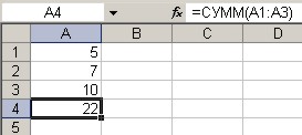
Enter arbitrary numbers in cells A1, A2, A3. Activate cell A4 and press the autosum button. The result is shown below.

Press the enter key. The formula for the sum of cells A1..A3 will be inserted into cell A4. The autosum button has a drop-down list from which you can select a different formula for the cell.

To select a function, use the Insert Function button in the formula bar. When pressed, the following window appears.

If you do not know exactly the function that you want to apply at the moment, you can search in the "Search for function" dialog box.

If the formula is very cumbersome, you can include spaces or line breaks in the formula text. This does not affect the calculation results in any way. To break a line, press the Alt + Enter key combination.

Using headings in formulas

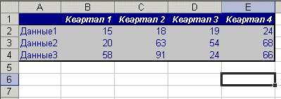
You can use table headers in formulas instead of referring to table cells. Build the following example.

By default, Microsoft Excel does not recognize headers in formulas. To use headings in formulas, choose Options on the Tools menu. On the Calculations tab, in the Book Options group, select the Allow Range Names check box.

In normal writing, the formula in cell B6 would look like this: \u003d SUM (B2: B4).

When using headers, the formula will look like this: \u003d SUM (Q1).

You need to know the following:

If the formula contains the column / row header it is in, then Excel assumes that you want to use the range of cells below the table column header (or to the right of the row header);

If the formula contains a column / row header that is different from the one it is in, Excel assumes that you want to use the cell at the intersection of the column / row with that header and the row / column where the formula is located.

When using headers, you can specify any cell in the table using - range intersection. For example, to reference cell C3 in our example, you can use the formula \u003d Row2 Kv 2. Notice the space between the row and column headings.

Formulas containing headings can be copied and pasted, and Excel automatically adjusts them to the columns and rows you want. If an attempt is made to copy the formula to an inappropriate place, Excel will inform you about this, and the cell will display the value NAME ?. When you change heading names, similar changes occur in the formulas.

«Data Entry in Excel || Excel || Excel cell names "

Cell and range names inExcel

- Names in formulas

- Assigning names in the name field

- Rules for naming cells and ranges

Excel cells and cell ranges can be named and then used in formulas. If formulas containing titles can be applied only in the same sheet as the table, then using the range names, you can refer to table cells anywhere in any workbook.

Names in formulas

The cell or range name can be used in a formula. Suppose we have the formula A1 + A2 written in cell A3. If you give cell A1 the name "Basis", and cell A2 - "Add-in", then the record Basis + Add-in will return the same value as the previous formula.

Assigning names to the name field

To assign a name to a cell (a range of cells), select the corresponding element, and then enter a name in the name field, while spaces cannot be used.

If a name has been given to the selected cell or range, then it is displayed in the name field, and not a reference to the cell. If a name is defined for a range of cells, it appears in the name field only when the entire range is selected.

If you want to navigate to a named cell or range, click the arrow next to the name field and select the cell or range name from the drop-down list.

More flexible possibilities of assigning names of cells and their ranges, as well as titles, are given by the "Name" command from the "Insert" menu.

Naming Rules for Cells and Ranges

The name must start with a letter, backslash (\\), or underscore (_).

Only letters, numbers, backslashes and underscores can be used in the name.

You cannot use names that can be interpreted as references to cells (A1, C4).

Single letters can be used as names, except for the letters R, C.

Spaces must be replaced with an underscore.

"Excel functions || Excel || ArraysExcel "

ArraysExcel

- Using arrays

- Two-dimensional arrays

- Rules for array formulas

Arrays in Excel are used to create formulas that return a set of results or operate on a set of values.

Using arrays

Let's look at a few examples in order to better understand arrays.

Let's calculate, using arrays, the sum of the row values \u200b\u200bfor each column. To do this, do the following:

Enter numeric values \u200b\u200bin the range A1: D2.

Highlight the range A3: D3.

In the formula bar, enter \u003d A1: D1 + A2: D2.

Press the key combination Ctrl + Shift + Enter.

Cells A3: D3 form an array range, and an array formula is stored in each cell in that range. Array of arguments are references to ranges A1: D1 and A2: D2

2D arrays

In the previous example, array formulas were placed in a horizontal, one-dimensional array. You can create arrays that contain multiple rows and columns. Such arrays are called two-dimensional.

Array Formula Rules

Before entering an array formula, you must select the cell or range of cells that will contain the results. If the formula returns multiple values, you must select a range that is the same size and shape as the original data range.

Press Ctrl + Shift + Enter to commit the array formula input. Excel will enclose the formula in curly braces in the formula bar. DO NOT INPUT THE FIGURE BRACKETS MANUALLY!

The range cannot be changed, cleared or moved individual cellsas well as insert or delete cells. All cells in the array range should be considered as a single whole and all of them should be edited at once.

To change or clear an array, select the entire array and activate the formula bar. After changing the formula, press the key combination Ctrl + Shift + Enter.

To move the contents of a range of an array, select the entire array and select the "Cut" command from the "Edit" menu. Then select the new range and choose Paste from the Edit menu.

You are not allowed to cut, clear, or edit part of the array, but you can assign different formats to individual cells in the array.

«Excel Cells and Ranges || Excel || Formatting in Excel "

Assigning and Deleting Formats inExcel

- Format assignment

- Format removal

- Formatting with toolbars

- Formatting individual characters

- Applying AutoFormat

Formatting in Excel is used to make data easier to read, which plays an important role in productivity.

Format assignment

Choose the command "Format" - "Cells" (Ctrl + 1).

In the dialog box that appears (the window will be discussed in detail later) enter the required formatting parameters.

Click the "Ok" button

A formatted cell retains its format until a new format is applied to it or an old one is removed. When you enter a value in a cell, the format already used in the cell is applied to it.

Format Removal

Select a cell (range of cells).

Choose Edit - Clear - Formats.

To delete values \u200b\u200bin cells, select the "All" command of the "Clear" submenu.

It should be borne in mind that when copying a cell, the format of the cell is also copied along with its content. This way, you can save time formatting the source cell before using the copy and paste commands.

Formatting with toolbars

The most frequently used formatting commands are moved to the "Formatting" toolbar. To apply the format using the toolbar button, select a cell or range of cells and then click the button. To delete the format, press the button again.

To quickly copy formats from selected cells to other cells, you can use the Format Painter button on the Formatting toolbar.

Formatting individual characters

Formatting can be applied to individual characters in a text value in a cell as well as to an entire cell. To do this, select the desired symbols and then in the "Format" menu, select the "Cells" command. Set the required attributes and click the "Ok" button. Press Enter to see the results of your work.

Applying AutoFormat

Excel automatic formats are predefined combinations of number format, font, alignment, border, pattern, column width, and line height.

To use autoformat, follow these steps:

Enter the required data into the table.

Select the range of cells you want to format.

From the Format menu, choose AutoFormat. This will open a dialog box.

In the AutoFormat dialog box, click the Options button to display the Modify area.

Select the appropriate auto format and click the "OK" button.

Select a cell outside the table to deselect the current block and you will see the formatting results.

«Excel arrays || Excel || Formatting numbers in Excel "

Formatting numbers and text in Excel

-General format

-Numeric formats

-Money formats

-Financial formats

-Percentage formats

- Fractional formats

-Exponential formats

-Text format

-Additional formats

-Creating new formats

The Format Cells dialog (Ctrl + 1) allows you to control the display of numeric values \u200b\u200band change the text output.

Before opening the dialog box, select the cell containing the number to be formatted. In this case, you will always see the result in the "Sample" field. Don't forget the distinction between stored and displayed values. The formats do not affect stored numeric or text values \u200b\u200bin cells.

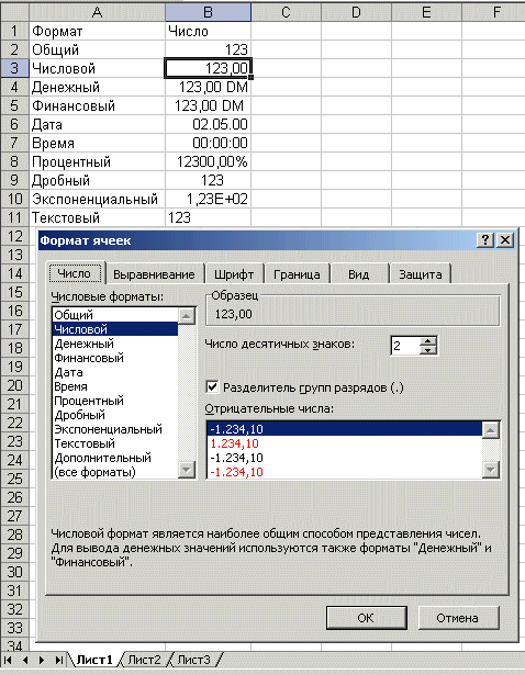
General format

Any text or numeric value entered is displayed in General format by default. At the same time, it is displayed exactly as it was entered in the cell, except for three cases:

Long numeric values \u200b\u200bare displayed in exponential notation or rounded off.

The format does not display trailing zeros (456.00 \u003d 456).

A decimal fraction entered without a number to the left of the decimal point is displayed with a zero (, 23 \u003d 0.23).

Number formats

This format allows you to display numeric values \u200b\u200bas integers or fixed-point numbers, and highlight negative numbers with color.

Monetary formats

These formats are similar to number formats, except that instead of a digit group separator, they control the display of the currency symbol, which you can select from the Designation list.

Financial formats

The financial format basically corresponds to the currency formats - you can display a number with or without a currency unit with a specified number of decimal places. The main difference is that the financial format displays the currency in a left-justified format, while the number itself is right-justified in the cell. As a result, both the currency and the numbers are vertically aligned in the column.

Percentage formats

This format displays numbers as percentages. The decimal point in the formatted number is shifted two digits to the right, and the percent sign is displayed at the end of the number.

Fractional formats

This format outputs fractional values \u200b\u200bas normal, not decimal fractions. These formats are especially useful when entering stock prices or measurements.

Exponential formats

Exponential formats display numbers in exponential notation. This format is very useful for displaying and outputting very small or very large numbers.

Text format

Applying a text format to a cell means that the value in that cell should be treated as text, as evidenced by the alignment to the left of the cell.

It doesn't matter if the numeric value is formatted as text, because Excel is capable of recognizing numeric values. An error will occur if there is a formula in a cell that has a text format. In this case, the formula is treated as plain text, so errors are possible.

Additional formats

Creation of new formats

To create a format based on an existing format, do the following:

Select the cells you want to format.

Press the key combination Ctrl + 1 and on the "Number" tab of the opened dialog window select the "All formats" category.

In the Type list, select the format you want to change and edit the contents of the field. The original format will remain unchanged, and the new format will be added to the "Type" list.

"Formatting in Excel || Excel ||

Aligning Excel Cell Contents

- Align left, center and right

-Filling cells

-Word wrap and justify

-Vertical alignment and text orientation

-Automatic character size

The Alignment tab of the Format Cells dialog box controls the placement of text and numbers in cells. You can also use this tab to create multi-line labels, repeat a series of characters in one or more cells, and change the orientation of text.

Align left, center and right

When you select Left, Center, or Right, the contents of the selected cells are aligned to the left, center, or right of the cell, respectively.

When aligning to the left, you can change the amount of indentation, which is assumed to be zero by default. Increasing the indent by one unit shifts the cell value one character to the right, which is approximately equal to the width of the Normal style capital X.

Filling the cells

Filled format repeats the value entered in the cell to fill the entire column width. For example, in the worksheet shown in the picture above, cell A7 repeats the word "Fill". Although the range of cells A7-A8 appears to contain many words "Padding", the formula bar suggests that there is actually only one word. Like all other formats, the Padded format only affects the appearance and not the stored content of the cell. Excel repeats characters along the entire range without gaps between cells.

It might seem that repeating characters are as easy to type with the keyboard as they are with filling. However, the Padded format has two important advantages. First, if you adjust the column width, Excel will increase or decrease the number of characters in the cell as appropriate. Secondly, you can repeat a character or characters in several adjacent cells at once.

Since this format affects numeric values \u200b\u200bin the same way as text, the number may not look the way it should. For example, if you apply this format to a 10-character-wide cell that contains the number 8, that cell will display 8888888888.

Word wrap and justification

If you enter a label that is too long for the active cell, Excel expands the label outside of the cell, provided the adjacent cells are empty. If you then select the Word Wrap check box on the Alignment tab, Excel displays this text entirely within one cell. To do this, the program will increase the height of the line the cell is in and then place the text on additional lines within the cell.

When using the "Fit to Width" horizontal alignment format, the text in the active cell is word-wrapped to additional lines within the cell and is aligned left and right with automatic line-height adjustment.

If you create a multi-line text box and subsequently clear the Word Wrap check box, or use a different horizontal alignment format, Excel restores the original line height.

The Justified vertical alignment format does essentially the same as its Justified counterpart, except that it aligns the cell value relative to its top and bottom edges, rather than the sides.

Vertical alignment and text orientation

Excel provides four vertical alignment formats for text: Top, Center, Bottom, and Height.

The Orientation area allows you to position the contents of cells vertically from top to bottom or tilted up to 90 degrees clockwise or counterclockwise. Excel automatically adjusts the row height in vertical orientation unless you manually or previously set the row height.

Autosize characters

The AutoFit checkbox reduces the size of the characters in the selected cell so that its contents fit completely in the column. This can be useful when working with a worksheet in which setting the column width to a long value has an undesirable effect on the rest of the data, or in that case. When using vertical or italic text, word wrap is not an acceptable solution. In the figure below, the same text has been entered in cells A1 and A2, but for cell A2 the "Auto-fit width" checkbox is selected. As the column width changes, the size of the characters in cell A2 will decrease or increase accordingly. However, this retains the font size assigned to the cell, and when the column width increases after reaching a certain value, the character size adjustment will not be performed.

It should be said that, although this format is a good way to solve some problems, it should be borne in mind that the size of characters can be as small as desired. If the column is narrow and the value is long enough, then after applying this format, the contents of the cell may become unreadable.

«Custom format || Excel || Font in Excel "

Using cell borders and fillsExcel

-Using borders

-Application of colors and patterns

-Using fill

Using boundaries

Borders and shading of cells can be a good way to decorate different areas of a worksheet or draw attention to important cells.

To select a line type, click on any of the thirteen border line types, including four solid lines of varying thickness, a double line, and eight types of dashed lines.

The default border line color is black if the Color field is set to Auto on the View tab of the Options dialog box. To select a color other than black, click the arrow to the right of the Color box. The current 56-color palette will open, in which you can use one of the available colors or define a new one. Note that you must use the Color list on the Border tab to select the border color. If you try to do this using the formatting toolbar, then change the text color in the cell, not the border color.

After choosing the type and color of the line, you need to specify the position of the border. When you click the Outside button in the All area, the border is placed around the perimeter of the current selection, be it a single cell or a block of cells. To remove all the borders in the selection, click the No button. The viewport allows you to control the placement of borders. When you first open a dialog box for a single selected cell, this area contains only small handles that indicate the corners of the cell. To place a border, click in the viewport where you want the border to be, or click the appropriate button next to that area. If several cells are selected in the worksheet, in this case, the "Internal" button becomes available on the "Border" tab, with which you can add borders between the selected cells. In addition, additional handles on the sides of the selection appear in the viewport to indicate where the inner borders will go.

To remove a placed border, simply click on it in the viewport. If you want to change the border format, select a different line type or color and click on that border in the preview area. If you want to start over placing borders, click the No button in the All area.

You can apply multiple border types to selected cells at the same time.

Combinations of borders can be applied using the Borders button on the Formatting toolbar. After clicking on the small arrow next to this button, Excel will bring up the Border Palette from which you can select the border type.

The palette consists of 12 border options, including combinations of different types, such as a single top border and a double bottom border. The first option in the palette removes all border formats in the selected cell or range. Other options show in miniature the location of the border or combination of borders.

As a practice, try the small example below. To break a line, press the Enter key while holding Alt.

Applying colors and patterns

Use the View tab of the Format Cells dialog box to apply color and patterns to the selected cells. This tab contains the current palette and a drop-down pattern palette.

The Color palette on the View tab lets you set the background for the selected cells. If you select a color in the Color palette without selecting a pattern, the specified background color will appear in the selected cells. If you select a color from the Color panel and then select a pattern from the Pattern drop-down panel, the pattern is superimposed on the background color. The colors in the Pattern drop-down palette control the color of the pattern itself.

Using fill

The different cell fill options provided by the View tab can be used to visually design the worksheet. For example, shading can be used to highlight data totals or to draw attention to cells in a worksheet for data entry. To make it easier to view numerical data line by line, you can use the so-called "strip fill", when lines of different colors alternate.

Select a background color for cells that makes it easy to read text and numeric values \u200b\u200bdisplayed in the default black font.

Excel allows you to add a background image to your worksheet. To do this, select the "Format" command, "Layout" - "Underlay". A dialog box will appear allowing you to open a graphic file stored on disk. This graphic is then used as the background of the current worksheet, like watermarks on a piece of paper. The graphic image is repeated if necessary until the entire worksheet is filled. You can turn off the display of grid lines in the sheet, for this, in the "Tools" menu, select the "Options" command and on the "View" tab and uncheck the "Grid" box. Cells that are assigned a color or pattern display only the color or pattern, not the background graphic.

«Excel Font || Excel || Merging cells "

Conditional formatting and merging of cells

- Conditional formatting

- Merge cells

- Conditional formatting

Conditional formatting allows you to apply formats to specific cells that remain dormant until the values \u200b\u200bin those cells reach some benchmark.

Select the cells intended for formatting, then in the "Format" menu, select the "Conditional Formatting" command, you will see the dialog box presented below.

The first combo box in the Conditional Formatting dialog box lets you choose whether the condition should be applied to the value or the formula itself. Typically, the Value option is selected, where the formatting depends on the values \u200b\u200bof the selected cells. The "Formula" parameter is used when you need to specify a condition that uses data from unselected cells, or you need to create a complex condition that includes several criteria. In this case, in the second combo box, you must enter a logical formula that takes on the value TRUE or FALSE. The second combo box is used to select the comparison operator used to specify the formatting condition. The third field is used to set the value to compare. If the operator "Between" or "Out" is selected, then an additional fourth field appears in the dialog window. In this case, the lower and upper values \u200b\u200bmust be specified in the third and fourth fields.

After specifying the condition, click the "Format" button. The Format Cells dialog box opens, where you can select the font, borders, and other format attributes to be applied when the specified condition is met.

In the example below, the format is set to font color red and font bold. Condition: if the value in the cell exceeds "100".

Sometimes it is difficult to determine where the conditional formatting has been applied. To select all conditionally formatted cells in the current sheet, choose Go from the Edit menu, click the Select button, then select the Conditional Formats radio button.

To remove a formatting condition, select a cell or range, and then choose Conditional Formatting from the Format menu. Specify the conditions you want to remove and click OK.

Merging cells

The grid is a very important design element of a spreadsheet. Sometimes it is necessary to format the mesh in a special way to achieve the desired effect. Excel allows you to merge cells, which gives the grid new features that you can use to create clearer forms and reports.

When cells are merged, one cell is formed, the dimensions of which coincide with the dimensions of the original selection. The merged cell gets the address of the top-left cell in the original range. The rest of the original cells practically cease to exist. If a formula contains a reference to such a cell, it is treated as empty, and depending on the type of formula, the reference may return a null or an error value.

To merge cells, do the following:

Select source cells;

In the "Format" menu, select the "Cells" command;

On the "Align" tab of the "Format Cells" dialog box, select the "Merge Cells" checkbox;

Click "OK".

If you have to use this command quite often, then it is much more convenient to "pull" it to the toolbar. To do this, select the "Service" - "Settings ..." menu, in the window that appears, go to the "Commands" tab and select the "Formatting" category in the right window. In the left window "Commands", using the scroll bar, find "Merge Cells" and drag this icon (using the left mouse button) to the "Formatting" toolbar.

Merging cells has a number of consequences, most notably the violation of grid, one of the main attributes of spreadsheets. In this case, some nuances should be taken into account:

If only one cell in the selected range is non-empty, then merging its contents is re-positioned in the merged cell. So, for example, when merging cells of the range A1: B5, where cell A2 is non-empty, this cell will be transferred to the merged cell A1;

If multiple cells in the selected range contain values \u200b\u200bor formulas, then the merge saves only the contents of the top left cell, which is re-positioned in the merged cell. The contents of the remaining cells are deleted. If you need to save data in these cells, then before merging, you should add them to the upper left cell or move to another location outside the selection;

If the merge range contains a formula that is repositioned in the merged cell, then the relative references in it are automatically adjusted;

United excel cellsyou can copy, cut and paste, delete and drag like regular cells. After you copy or move the merged cell, it occupies the same number of cells in the new location. In place of the cut or deleted merged cell, the standard cell structure is restored;

When you merge cells, all borders are removed, except for the outer border of the entire selection, as well as the border that is applied to any edge of the entire selection.

"Borders and Shading || Excel || Editing"

Cutting and pasting cells inExcel

Cut and Paste

Cut and Paste Rules

Inserting cut cells

Cut and Paste

You can use the Cut and Paste commands on the Edit menu to move values \u200b\u200band formats from one location to another. Unlike the Delete and Clear commands, which delete cells or their contents, the Cut command places a movable dotted box around the selected cells and places a copy of the selection on the clipboard, which saves the data so that it can be pasted into another place.

After selecting the range in which you want to move the cut cells, the "Paste" command places them in a new location, clears the contents of the cells inside the movable frame and removes the movable frame.

When you use the Cut and Paste commands to move a range of cells, Excel clears the content and formats in the cut range and brings them to the paste range.

Excel adjusts any formulas outside the clipping region that reference these cells.

Cut and Paste Rules

The selected clipping area must be a single rectangular block of cells;

The Cut command inserts only one time. To paste the selected data into several places, use the "Copy" - "Clear" command combination;

You do not have to select the entire insert range before using the Paste command. When you select one cell as the paste range, Excel expands the paste area to fit the size and shape of the clip area. The selected cell is considered the upper left corner of the insertion area. If you select the entire area of \u200b\u200bthe paste, then you need to make sure that the selected range is the same size as the area to be cut;

When you use the Paste command, Excel replaces the content and formats in all existing cells in the paste range. If you do not want to lose the contents of existing cells, make sure there are enough blank cells below and to the right of the selected cell, which will end up in the upper left corner of the screen area, to accommodate the entire clipping area in the worksheet.

Inserting cut cells

When you use the Paste command, Excel inserts the cut cells into the selected area of \u200b\u200bthe worksheet. If the selection already contains data, it is replaced by the inserted values.

In some cases, you can paste the contents of the clipboard between cells instead of placing it in existing cells. To do this, use the Cut Cells command on the Insert menu instead of the Paste command on the Edit menu.

The "Cut Cells" command replaces the "Cells" command and appears only after the data is deleted to the clipboard.

For example, in the example below, cells A5 were originally cut: A7 (the Cut command of the Edit menu); then cell A1 was made active; then the "Cut Cells" command from the "Insert" menu is executed.

«Filling rows || Excel || Excel functions "

Functions. Function syntaxExcel

Function syntax

Using arguments

Argument types

In lesson # 4, we already made our first acquaintance with Excel functions. Now is the time to take a closer look at this powerful spreadsheet toolkit.

Excel functions are special, pre-built formulas that allow you to quickly and easily perform complex calculations. They can be compared to the special keys on calculators for calculating square roots, logarithms, etc.

Excel has several hundred built-in functions that perform a wide variety of different calculations. Some functions are the equivalent of long mathematical formulas that you can do yourself. And some functions cannot be implemented in the form of formulas.

Function syntax

Functions have two parts: the function name and one or more arguments. A function name, such as SUM, describes the operation that this function performs. Arguments specify the values \u200b\u200bor cells used by the function. In the formula below: SUM - function name; B1: B5 is an argument. This formula sums up the numbers in cells B1, B2, B3, B4, B5.

SUM (B1: B5)

An equal sign at the beginning of a formula means that you entered the formula, not the text. If there is no equal sign, Excel will treat the input as just text.

The function argument is enclosed in parentheses. An open parenthesis marks the beginning of an argument and appears immediately after the function name. If you enter a space or other character between the name and the opening parenthesis, the cell will display an erroneous value #NAME? Some functions have no arguments. Even so, the function must contain parentheses:

Using arguments

When using multiple arguments in a function, they are separated from one another by semicolons. For example, the following formula indicates that you need to multiply the numbers in cells A1, A3, A6:

PRODUCT (A1; A3; A6)

A function can use up to 30 arguments, as long as the total length of the formula does not exceed 1024 characters. However, any argument can be a range containing an arbitrary number of sheet cells. For instance:

Argument types

In the previous examples, all arguments were cell or range references. However, you can also use numeric, text, and boolean values, range names, arrays, and error values \u200b\u200bas arguments. Some functions return values \u200b\u200bof these types, and they can later be used as arguments in other functions.

Numerical values

Function arguments can be numeric. For example, the SUM function in the following formula adds the numbers 24, 987, 49:

SUM (24; 987; 49)

Text values

Text values \u200b\u200bcan be used as a function argument. For instance:

TEXT (TDATA (); "D MMM YYYY")

In this formula, the second argument to the TEXT function is text and specifies a template for converting the decimal date value returned by the TDATA function (NOW) to a character string. The text argument can be a character string enclosed in double quotes, or a reference to a cell that contains text.

Boolean values

Arguments of some functions can only accept the logical values \u200b\u200bTRUE or FALSE. A Boolean expression returns TRUE or FALSE to the cell or formula that contains the expression. For instance:

IF (A1 \u003d TRUE; "Increase"; "Decrease") & "prices"

You can specify a range name as an argument to the function. For example, if the name "Debit" (Insert-Name-Assign) is assigned to the range of cells A1: A5, then the formula can be used to calculate the sum of the numbers in cells A1 through A5

SUM (Debit)

Using different types of arguments

Arguments of different types can be used in one function. For instance:

AVERAGE (Debit; C5; 2 * 8)

«Inserting cells || Excel || Entering Excel Functions "

Entering functions in a worksheetExcel

You can enter functions in a worksheet directly from the keyboard or using the Function command of the Insert menu. When entering a function from the keyboard, it is better to use lower case... When you finish entering a function, Excel will change the letters in the function name to uppercase if it was entered correctly. If the letters do not change, then the function name is entered incorrectly.

If you select a cell and choose "Function" from the "Insert" menu, Excel displays the "Function Wizard" dialog box. This can be achieved a little faster by pressing the function icon key in the formula bar.

You can also open this window using the "Insert Function" button on the standard toolbar.

In this window, first select a category from the Category list and then select the desired function in the Function alphabetical list.

Excel will enter an equal sign, a function name, and a pair of parentheses. Then Excel will open a second dialog box of the Function Wizard.

The second dialog box of the Function Wizard contains one field for each argument of the selected function. If the function has a variable number of arguments, this dialog box expands when additional arguments are given. The description of the argument whose field contains the insertion point is displayed at the bottom of the dialog box.

To the right of each argument field, its current value is displayed. This is very handy when you are using links or names. The current value of the function is displayed at the bottom of the dialog box.

Click the "OK" button and the created function will appear in the formula bar.

"Function syntax || Excel || Mathematical functions "

Math functionsExcel

The most commonly used Excel math functions are covered here (quick reference). More information about functions can be found in the Function Wizard dialog box as well as in the Excel help system. In addition, many math functions are included in the Analysis Package add-in.

SUM function

Functions EVEN and ODD

Functions OKRVNIZ, OKRVVERKH

Functions WHOLE and OTBR

Functions RAND and RAND BETWEEN

PRODUCT function

OSTAT function

ROOT function

NUMBER COMB function

ISNUMBER function

LOG function

LN function

EXP function

PI function

RADIANS and DEGREES function

SIN function

COS function

TAN function

SUM function

The SUM function adds a set of numbers. This function has the following syntax:

SUM (numbers)

The number argument can contain up to 30 elements, each of which can be a number, formula, range, or a reference to a cell containing or returning a numeric value. The SUM function ignores arguments that refer to empty cells, text, or boolean values. Arguments do not have to form contiguous ranges of cells. For example, to get the sum of the numbers in cells A2, B10, and cells C5 through K12, enter each reference as a separate argument:

SUM (A2; B10; C5: K12)

Functions ROUND, ROUNDDOWN, ROUNDUP

The ROUND function rounds the number given by its argument to a specified number of decimal places and has the following syntax:

ROUND (number; num_digits)

The number argument can be a number, a reference to the cell that contains the number, or a formula that returns a numeric value. The num_digits argument, which can be any positive or negative integer, specifies how many digits to round. Specifying a negative num_digits argument rounds to the specified number of digits to the left of the decimal point, and setting num_digits to 0 rounds to the nearest integer. Excel numbers that are less than 5 are with a downside (down), and numbers that are greater than or equal to 5 are with an excess (up).

The functions ROUNDDOWN and ROUNDUP have the same syntax as the ROUND function. They round values \u200b\u200bdown (under) or up (over).

Functions EVEN and ODD

You can use the EVEN and ODD functions to perform rounding operations. The EVEN function rounds a number up to the nearest even integer. The ODD function rounds a number up to the nearest odd integer. Negative numbers are rounded down, not up. Functions have the following syntax:

EVEN (number)

ODD (number)

Functions OKRVNIZ, OKRVVERKH

The functions FLOOR and CEILING can also be used to perform rounding operations. The FLOOR function rounds a number down to the nearest multiple of the specified factor, and the OKRVNIZ function rounds the number up to the nearest multiple of the specified factor. These functions have the following syntax:

FLOOR (number; multiplier)

OKRVVERH (number; multiplier)

The number and multiplier values \u200b\u200bmust be numeric and have the same sign. If they have different signs, an error will be generated.

Functions WHOLE and OTBR

The INT function rounds a number down to the nearest integer and has the following syntax:

INT (number)

The number argument is the number for which you want to find the next smallest integer.

Consider the formula:

WHOLE (10,0001)

This formula will return 10, just like the following:

WHOLE (10,999)

The TRUNC function truncates all digits to the right of the decimal point, regardless of the sign of the number. The optional argument num_digits specifies the position after which to truncate. The function has the following syntax:

OST (number; number_digits)

If the second argument is omitted, it is assumed to be zero. The following formula returns 25:

OTBR (25,490)

The ROUND, INT, and CUT functions remove unnecessary decimal places, but they work differently. The ROUND function rounds up or down to a specified number of decimal places. The INT function rounds down to the nearest whole number, and the OPT function discards the decimal places without rounding. The main difference between the INTEGER and CLEAR functions is in the handling of negative values. If you use the value -10.900009 in the INT function, the result is -11, but if you use the same value in the OPT function, the result is -10.

Functions RAND and RAND BETWEEN

The RAND function generates random numbers evenly spaced between 0 and 1 and has the following syntax:

The RAND function is one of the EXCEL functions that have no arguments. As with all functions that have no arguments, you must enter parentheses after the function name.

The value of the RAND function changes every time the sheet is recalculated. If automatic update of calculations is set, the value of the RAND function changes every time you enter data in this sheet.

The RANDBETWEEN function, which is available when the Analysis Package add-in is installed, provides more options than RAND. For the RANDBETWEEN function, you can set the interval of the generated random integer values.

Function syntax:

RANDBETWEEN (start; end)

The start argument is the smallest integer that can return any integer between 111 and 529 (including both):

RANDBETWEEN (111; 529)

PRODUCT function

The PRODUCT function multiplies all numbers given by its arguments and has the following syntax:

PRODUCT (number1, number2 ...)

This function can have up to 30 arguments. Excel will ignore any blank cells, text and boolean values.

OSTAT function

The REST function (MOD) returns the remainder of a division and has the following syntax:

OSTAT (number; divisor)

The value of the OSTAT function is the remainder obtained by dividing the argument number by the divisor. For example, the following function will return 1, the remainder of 19 divided by 14:

OSTAT (19; 14)

If the number is less than the divisor, then the function value is equal to the number argument. For example, the following function will return 25:

OSTAT (25; 40)

If the number is exactly divisible by the divisor, the function returns 0. If the divisor is 0, the OSTAT function returns an error value.

ROOT function

The ROOT (SQRT) function returns the positive square root of a number and has the following syntax:

ROOT (number)

Number must be a positive number. For example, the following function returns 4:

ROOT (16)

If the number is negative, ROOT returns an error value.

NUMBER COMB function

The COMBIN function determines the number of possible combinations or groups for a given number of items. This function has the following syntax:

COMBIN (number, number_selected)

Number is the total number of items, and num_selected is the number of items in each combination. For example, to determine the number of 5-player teams that can be formed from 10 players, use the formula:

NUMBER COMB (10; 5)

The result will be 252. That is, 252 teams can be formed.

ISNUMBER function

The ISNUMBER function determines whether a value is a number and has the following syntax:

ISNUMBER (value)

Suppose you want to know if the value in cell A1 is a number. The following formula returns TRUE if cell A1 contains a number or a formula that returns a number; otherwise, it returns FALSE:

ISNUMBER (A1)

LOG function

The LOG function returns the logarithm of a positive number to a specified base. Syntax:

LOG (number; base)

If radix is \u200b\u200bnot specified, Excel assumes it is 10.

LN function

The LN function returns the natural logarithm of the positive number specified as an argument. This function has the following syntax:

EXP function

The EXP function calculates the value of a constant raised to a given power. This function has the following syntax:

EXP function is the inverse of LN. For example, suppose cell A2 contains the formula:

Then the following formula returns 10:

PI function

The PI function returns the value of the constant pi with precision to 14 decimal places. Syntax:

RADIANS and DEGREES function

Trigonometric functions use angles expressed in radians, not degrees. The measurement of angles in radians is based on the constant pi, and 180 degrees are equal to pi radians. Excel provides two functions, RADIANS and DEGREES, to make it easier to work with trigonometric functions.

You can convert radians to degrees using the DEGREES function. Syntax:

DEGREES (angle)

Here - angle is a number representing the angle measured in radians. To convert degrees to radians, use the RADIANS function, which has the following syntax:

RADIANS (angle)

Here - angle is a number representing the angle measured in degrees. For example, the following formula returns 180:

DEGREES (3.14159)

At the same time, the following formula returns 3.14159:

RADIANS (180)

SIN function

The SIN function returns the sine of an angle and has the following syntax:

SIN (number)

COS function

The COS function returns the cosine of an angle and has the following syntax:

COS (number)

Here the number is the angle in radians.

TAN function

The TAN function returns the tangent of an angle and has the following syntax:

TAN (number)

Here the number is the angle in radians.

«Entering functions || Excel || Text functions "

Text functionsExcel

Here are some of the most commonly used text functions in Excel (quick reference). More information about functions can be found in the Function Wizard dialog box as well as in the Excel help system.

TEXT function

RUBLE function

DLSTR function

SYMBOL and CODE function

Functions JSPROBEL and PECHSIMV

EXACT function

ETEXT and ENETEXT functions

Text functions convert numeric text values \u200b\u200bto numbers and numeric values \u200b\u200bto character strings (text strings), and also allows you to perform various operations on character strings.

TEXT function

The TEXT function converts a number to a text string with the specified format. Syntax:

TEXT (value; format)

The value argument can be any number, formula, or cell reference. The format argument determines how the returned string is displayed. You can use any of the formatting characters except the asterisk to specify the format you want. The use of the General format is not allowed. For example, the following formula returns the text string 25.25:

TEXT (101/4; "0.00")

RUBLE function

The DOLLAR function converts a number to a string. However, RUBLE returns a currency string with a specified number of decimal places. Syntax:

RUBLE (number; number_signs)

Excel rounds the number if necessary. If num_chars is omitted, Excel uses two decimal places, and if this argument is negative, the return value is rounded to the left of the decimal point.

DLSTR function

The DLSTR (LEN) function returns the number of characters in a text string and has the following syntax:

DLSTR (text)

The text argument must be a character string, enclosed in double quotes, or a cell reference. For example, the following formula returns 6:

DLSTR ("head")

The DLSTR function returns the length of the displayed text or value, not the stored cell value. It also ignores non-significant zeros.

SYMBOL and CODE function

Any computer uses numeric codes to represent characters. The most common character encoding system is ASCII. In this system, numbers, letters, and other symbols are represented by numbers from 0 to 127 (255). Functions CHAR and CODE deal with ASCII codes. The SYMBOL function returns the character that matches the specified numeric ASCII code, and the CODE function returns the ASCII code for the first character of its argument. Function syntax:

SYMBOL (number)

CODE (text)

If you enter a character as an argument, be sure to enclose it in double quotes, otherwise Excel will return an erroneous value.

Functions JSPROBEL and PECHSIMV

Often times, leading and trailing spaces prevent the values \u200b\u200bfrom being sorted correctly in a worksheet or database. If you use text functions to work with worksheet texts, extra spaces can prevent formulas from working properly. The TRIM function removes leading and trailing spaces from a string, leaving only one space between words. Syntax:

TRIM (text)

The CLEAN function is similar to the TRIM function except that it removes all non-printable characters. The PRINT function is especially useful when importing data from other programs because some imported values \u200b\u200bmay contain non-printable characters. These symbols may appear on worksheets as small squares or vertical bars. The PRINT function allows you to remove non-printable characters from such data. Syntax:

PECHSIMV (text)

EXACT function

The EXACT function compares two lines of text for complete identity, case-sensitive. The difference in formatting is ignored. Syntax:

COUNCIL (text1; text2)

If text1 and text2 are case-sensitive, the function returns TRUE; otherwise, FALSE. The text1 and text2 arguments must be character strings enclosed in double quotes or references to cells that contain text.

Functions UPPER, LOWER and PROPNACH

Excel has three functions that allow you to change the case of letters in text strings: UPPER, LOWER, and PROPER. The UPPER function converts all letters in a text string to uppercase, and LOWER to lowercase. The PROPER function capitalizes the first letter in each word and all letters immediately following non-letter characters; all other letters are converted to lowercase. These functions have the following syntax:

UPPER (text)

LOWER (text)

PROPNACH (text)

When working with already existing data, a situation often arises when you need to modify the original values \u200b\u200bthemselves, to which text functions are applied. You can enter the function in the same cells as these values, as the entered formulas will override them. But you can create temporary formulas with a text function in free cells in the same row and copy the result to the clipboard. To replace the original values \u200b\u200bwith the modified ones, select the original cells with the text, choose the Paste Special command from the Edit menu, select the Values \u200b\u200bradio button, and click OK. You can then delete temporary formulas.

ETEXT and ENETEXT functions

The ISTEXT and ISNOTEXT functions check if a value is text. Syntax:

ETEXT (value)

ENETEXT (value)

Suppose you want to determine if the value in cell A1 is text. If cell A1 contains text or a formula that returns text, you can use the formula:

ETEXT (A1)

In this scenario, Excel returns the Boolean value TRUE. Similarly, if you use the formula:

ENETEXT (A1)

Excel returns the Boolean value FALSE.

«Mathematical functions || Excel || String functions "

FunctionsExcel to work with line items

FIND and SEARCH functions

Functions RIGHT and LEFT

PSTR function

REPLACE and SUBSTITUTE functions

REPEAT function

CONCATENATE function

The following functions find and return parts of text strings or make large strings from small ones: FIND, SEARCH, RIGHT, LEFT, MID, SUBSTITUTE, REPT, REPLACE, CONCATENATE.

FIND and SEARCH functions

The FIND and SEARCH functions are used to determine the position of one text string in another. Both functions return the character number from which the first occurrence of the search string begins. These two functions work the same way, except that FIND is case-sensitive and SEARCH accepts wildcard characters. Functions have the following syntax:

FIND (lookup_text; lookup_text; start_position)

SEARCH (lookup_text; lookup_text; start_position)

Lookup_text is the text string to find, and lookup_text is the text to search for. Any of these arguments can be a character string, enclosed in double quotes, or a cell reference. The optional argument start_num specifies the position in the text being viewed at which to start the search. The start_num argument should be used when the lookup_text contains multiple occurrences of the search text. If this argument is omitted, Excel returns the position of the first occurrence.

These functions return an error value when lookup_text is not contained in the text being searched, or start_position is less than or equal to zero, or start_position is greater than the number of characters in the text being looked up, or start_position is greater than the position of the last occurrence of the searched text.

For example, to determine the position of the letter "g" in the line "Garage doors", you must use the formula:

FIND ("f"; "Garage doors")

This formula returns 5.

If you do not know the exact character sequence of the text you are looking for, you can use the SEARCH function and include the wildcard characters in the search_text string: a question mark (?) And an asterisk (*). A question mark matches one randomly typed character, and an asterisk replaces any sequence of characters at the specified position. For example, to find the position of the names Anatoly, Alexey, Akaki in the text located in cell A1, you need to use the formula:

SEARCH ("A * d"; A1)

Functions RIGHT and LEFT

The RIGHT function returns the rightmost characters in the argument string, while the LEFT function returns the first (left) characters. Syntax:

RIGHT (text; num_chars)

LEFT (text; num_chars)

The num_characters argument specifies the number of characters to extract from the text argument. These functions are whitespace-aware, and therefore, if the text argument contains leading or trailing whitespace, the TRIM function should be used in the function arguments.

Num_chars must be greater than or equal to zero. If this argument is omitted, Excel considers it to be 1. If the number of characters is greater than the number of characters in the text argument, the entire argument is returned.

PSTR function

The MID function returns a specified number of characters from a string of text, starting at a specified position. This function has the following syntax:

MID (text; start_num; num_chars)

The text argument is a text string containing the characters to be extracted, start_num is the position of the first character to be extracted from the text (relative to the beginning of the line), and num_chars is the number of characters to be extracted.

REPLACE and SUBSTITUTE functions

These two functions replace characters in text. The REPLACE function replaces part of a text string with another text string and has the syntax:

REPLACE (old_text; start_position; number of characters; new_text)

Old_text is the text string to replace characters with. The next two arguments specify the characters to be replaced (relative to the beginning of the line). The new_text argument specifies the text string to insert.

For example, cell A2 contains the text "Vasya Ivanov". To put the same text in cell A3, replacing the name, you need to insert the following function into cell A3:

REPLACE (A2; 1; 5; "Petya")

In the SUBSTITUTE function, the starting position and the number of characters to be replaced are not specified, but the replacement text is explicitly specified. The SUBSTITUTE function has the following syntax:

SUBSTITUTE (text; old_text; new_text; occurrence_number)

Entry_number is optional. It tells Excel to replace only the specified occurrence of the string old_text.

For example, cell A1 contains the text "Zero less than eight". It is necessary to replace the word "zero" with "zero".

SUBSTITUTE (A1; "o"; "y"; 1)

The number 1 in this formula indicates that only the first "o" in the row of cell A1 needs to be changed. If occurrence_num is omitted, Excel replaces all occurrences of old_text with new_text.

REPEAT function

The REPT function allows you to fill a cell with a string of characters repeated a specified number of times. Syntax:

REPEAT (text, repetitions)

The text argument is the multiplied character string, enclosed in quotation marks. The repeat_number argument specifies how many times to repeat the text. If repetition_num is 0, the REPEAT function leaves the cell blank, and if it is not an integer, this function strips the decimal places after the decimal point.

CONCATENATE function

The CONCATENATE function is the equivalent of the textual & operator and is used to concatenate strings. Syntax:

CONCATENATE (text1; text2; ...)

You can use up to 30 arguments in a function.

For example, cell A5 contains the text "first half of the year", the following formula returns the text "Total for the first half of the year":

CONCATENATE ("Total for"; A5)

«Text functions || Excel || Logic functions "

Logic functionsExcel

IF function

Functions AND, OR, NOT

Nested IF functions

Functions TRUE and FALSE

ISBLANK function

Boolean expressions are used to write conditions that compare numbers, functions, formulas, text, or Boolean values. Any Boolean expression must contain at least one comparison operator that defines the relationship between the elements of the Boolean expression. Below is a list of operators excel comparisons

\u003e More

< Меньше

\u003e \u003d Greater than or equal

<= Меньше или равно

<> Not equal

The result of a Boolean expression is the logical value TRUE (1) or the logical value FALSE (0).

IF function

The IF function has the following syntax:

IF (boolean_expression; value_if_true; value_if_false)

The following formula returns 10 if the value in cell A1 is greater than 3 and 20 otherwise:

IF (A1\u003e 3; 10; 20)

Other functions can be used as arguments to the IF function. You can use text arguments in the IF function. For instance:

IF (A1\u003e \u003d 4; "Passed the test"; "Did not pass the test")

You can use text arguments in the IF function so that if a condition is not met, it returns an empty string instead of 0.

For instance:

IF (SUM (A1: A3) \u003d 30; A10; "")

The logical_expression argument to the IF function can contain a text value. For instance:

IF (A1 \u003d Dynamo; 10; 290)

This formula returns 10 if cell A1 contains the string Dynamo, and 290 if it contains any other value. The match between the text values \u200b\u200bbeing compared must be exact, but not case sensitive. AND, OR, NOT Functions

Functions AND (AND), OR (OR), NOT (NOT) - allow you to create complex logical expressions. These functions work in conjunction with simple comparison operators. The AND and OR functions can take up to 30 boolean arguments and have the syntax:

AND (boolean1; boolean2 ...)

OR (boolean_value1, boolean_value2 ...)

The function does NOT have only one argument and the following syntax:

NOT (boolean_value)

Arguments of AND, OR, NOT functions can be logical expressions, arrays, or references to cells containing logical values.

Let's give an example. Let Excel return the text "Passed" if the student has a GPA of more than 4 (cell A2) and skipping classes is less than 3 (cell A3). The formula will take the form:

IF (AND (A2\u003e 4; A3<3);"Прошел";"Не прошел")

Despite the fact that the OR function has the same arguments as the AND, the results are completely different. So, if in the previous formula replace the AND function with OR, then the student will pass if at least one of the conditions is met (the average score is more than 4 or the absence of classes is less than 3). Thus, the OR function returns the logical value TRUE if at least one of the logical expressions is true, and the AND function returns the logical value TRUE only if all the logical expressions are true.

A function does NOT change the value of its argument to the opposite boolean value and is usually used in conjunction with other functions. This function returns the Boolean value TRUE if the argument is FALSE, and the Boolean value FALSE if the argument is TRUE.

Nested IF functions

Sometimes it is very difficult to solve a logic problem only with the help of comparison operators and functions AND, OR, NOT. In these cases, you can use nested IF functions. For example, the following formula uses three IF functions:

IF (A1 \u003d 100; "Always"; IF (AND (A1\u003e \u003d 80; A1<100);"Обычно";ЕСЛИ(И(А1>\u003d 60; A1<80);"Иногда";"Никогда")))

If the value in cell A1 is an integer, the formula reads as follows: "If the value in cell A1 is 100, return the string Always. Otherwise, if the value in cell A1 is between 80 and 100, return Usually." Otherwise, if the value in cell A1 is between 60 and 80, return the string “Sometimes.” And, if none of these conditions are met, return the string “Never.” Up to 7 levels of nesting of IF functions are allowed.

Functions TRUE and FALSE

The TRUE and FALSE functions provide an alternative way to write the logical values \u200b\u200bTRUE and FALSE. These functions have no arguments and look like this:

For example, cell A1 contains a boolean expression. Then the following function will return the value "Pass" if the expression in cell A1 is TRUE:

IF (A1 \u003d TRUE (), "Go through", "Stop")

Otherwise, the formula will return "Stop".

ISBLANK function

If you need to determine if a cell is empty, you can use the ISBLANK function, which has the following syntax:

ISBLANK (value)

“String functions || Excel || Excel 2007 "