Function to compare two columns in excel. How to compare two columns in Excel - Excel data comparison methods
Instructions
Use the built-in COUNTIF cell comparison function if you want to compare text values \u200b\u200bin table column cells with sample text and recalculate all that match. Start by filling a column with text values, and then in another column, click the cell where you want to see the counting result and enter the appropriate formula. For example, if the checked values \u200b\u200bare in column A, and the result should be placed in the first cell of column C, then its content should be as follows: \u003d COUNTIF ($ A: $ A; "Grape") Here "Grape" is a string value with which the values \u200b\u200bof all cells in column A are compared. You can skip specifying it in the formula, but place it in a separate cell (for example - in B1) and insert the corresponding link into the formula: \u003d COUNTIF ($ A: $ A; B1)
Use options conditional formattingif you need to visually highlight the result of comparing string variables in the table. For example, if you need to select cells in column A, the text of which matches the pattern in cell B1, then start by selecting this column - click its heading. Then click the Conditional Formatting button in the Styles command group on the Home tab on the Excel menu. Go to the "Cell Selection Rules" section and select the "Equals" line. In the window that opens, specify a sample cell (click cell B1) and select an option for matching rows from the drop-down list. Then click the "OK" button.
Use a combination of the built-in IF and CONCATENATE functions when you need to match more than one text cell to a pattern. The CONCATENATE function concatenates the values \u200b\u200bit specifies into one string variable. For example, the command CONCATE (A1; "and"; B1) will add the text "and" to the row from cell A1, and after it will place the row from cell B1. The string constructed in this way can then be compared against the pattern using the IF function. When you need to compare more than one string, it is more convenient to give your own name to the sample cell. To do this, click it and to the left of strings formulas, instead of a cell name (for example, C1), type its new name (for example, "sample"). Then click the cell in which the comparison result should be and enter the formula: IF (CONCATENATE (A1; "and"; B1) \u003d sample; 1; 0) Here unit is the value that the cell with the formula will contain if the comparison will give a positive result and zero for a negative result. Multiply this formula for everything strings tables that need to be compared with the sample is very simple - move the cursor to the lower right corner of the cell and when the cursor changes (becomes a black cross), press the left mouse button and drag this cell down to the last one to be compared strings.
If you work with spreadsheet documents large volume (many data / columns), it is very difficult to control the reliability / relevance of all information. Therefore, it is very often required to analyze two or more columns in an Excel document for duplicate detection. And if the user does not have information about all the functionality of the program, he may logically have a question: how to compare two columns in excel?
The answer has long been invented by the developers of this program, who initially laid down commands in it to help compare the information. In general, if you go into the depths of this issue, you can find about a dozen different ways, including writing individual macros and formulas. But practice shows: it is enough to know three or four reliable ways to cope with the emerging needs in comparison.
How to compare two columns in excel for matches
Data in Excel is usually compared between rows, between columns, with the value specified as a reference. If you need to compare columns, you can use the built-in functionality, namely, the "Match" and "If" actions. And all you need is Excel not earlier than the seventh year of "release".
We start with the function "Match". For example, the data being compared is in columns with addresses C3 and B3. The result of the comparison must be placed in a box, for example, D3. We click on this cell, enter the "formulas" menu directory, find the "function library" line, open the functions placed in the drop-down list, find the word "text" and click on "Match".
In a moment, you will see a new form on the display, where there will be only two fields: "text one", "text two". It is necessary to score in them, just, the addresses of the compared columns (C3, B3), then click on the familiar "OK" button. As a result, you will see the result with the words "True" / "False". In principle, nothing too complicated even for a novice user! But this is far from the only method. Let's take a look at the If function.
Ability to compare two columns in excel for matches using "If" allows you to enter values \u200b\u200bthat will be displayed as a result after the operation. The cursor is placed in the cell where the input will be carried out, the menu directory “library of functions” opens, the line “logical” is selected in the drop-down list, in which the first position will be occupied by the command “If”. We choose it.
Next, a form of reasoned filling takes off. "Log_Expression" is the formulation of the function itself. In our case, this is a comparison of two columns, so we enter "B3 \u003d C3" (or your column addresses). Further fields "value_if true", "value_if_false". Here you should enter the data (labels / words / numbers) that must correspond to a positive / negative result. After filling, we press, as usual, "ok". Let's get acquainted with the result.
If you need to perform a line-by-line analysis of two columns, in the third column we place any function that was discussed above ("if" or "coincide"). We extend its action to the entire height of the filled columns. Next, select the third column, click the "home" tab, look for the word "styles" in the group that appears. The "Column / Cell Selection Rules" will open.
In them you need to select the command "equal", then click on the first column and click on "Enter". As a result, it turns out to "tint" the columns where there are matching results. And you will immediately see the information you need. Further, in the analysis of the topic "how to compare the values \u200b\u200bof two columns in excel", we will move on to such a method as conditional formatting in Excel.
Excel: Conditional Formatting
Conditional formatting will allow you not only to compare two different columns / cells / lines, but also to highlight different data in them in a given color (red). That is, we are looking not for coincidences, but for differences. To get it, we act like this. Select the required columns without touching their names, go to the "main" menu directory, find the "styles" subsection in it.
It will contain the string "conditional formatting". By clicking on it, we get a list where we need a "create rule" item-function. The next step: in the line "format" you need to drive in the formula \u003d $ A2<>$ B2. This formula will help Excel understand exactly what we need, namely, to color in red all the values \u200b\u200bin column A that do not equal the values \u200b\u200bin column B. A slightly more complex way of applying formulas relates to the participation of constructs such as HLOOKUP / VLOOKUP. These formulas refer to horizontal / vertical search for values. Let's consider this method in more detail.
HLOOKUP and VLOOKUP
These two formulas allow you to search for data horizontally / vertically. That is, H is the horizontal, and V is the vertical. If the data to be compared is in the left column relative to the one where the compared values \u200b\u200bare located, use the VLOOKUP construction. But if the data for comparison is located horizontally at the top of the table from the column where the reference values \u200b\u200bare indicated, we use the HLOOKUP construction.
To understand how to compare data in two excel columns vertically, you should use this complete formula: lookup_value, table_array, col_index_num, range_lookup.
The value to be found is denoted as "lookup_value". Search columns are driven in like "table array". The column number should be specified as "col_index_num". Moreover, this is the column, the value of which coincided, and which needs to be returned / corrected. The range lookup command is optional here. It can indicate whether the value needs to be made accurate or approximate.
If this command is not specified, values \u200b\u200bwill be returned for both types. The entire HLOOKUP formula looks like this: lookup_value, table_array, row_index_num, range_lookup. Working with it is almost identical to the one described above. True, there is an exception. This is the line index that defines the line whose values \u200b\u200bshould be returned. If you learn how to clearly apply all of the above methods, it becomes clear: there is no more convenient and universal program for working with a large amount of data of different types than Excel. Comparing two columns in excel is, however, only half the job. After all, something else needs to be done with the obtained values. That is, the found matches still need to be processed somehow.
Method of handling duplicate values
So, there are found numbers in the first, suppose, column, completely repeating in the second column. It is clear that manually correcting repetitions is an unreal work that takes a lot of precious time. Therefore, you should use a ready-made technique for automatic correction.
For this to work, you first need to name the columns if they don't exist. Adjust the cursor to the first line, right-click, select "paste" in the menu that appears. Let's say the titles are "name" and "duplicate". Next, you need the directory "date", in it - "filter". Click on the tiny arrow next to the "duplicate" and remove all the "birds" from the list. Now click "ok", and the duplicate values \u200b\u200bin column A become visible.
Next, we select these cells, because we needed not only to compare the text in two columns in excel, but also to remove duplicates. We selected, right-clicked, selected “delete row”, clicked “ok” and got a table without matching values. The method works if the columns are on the same page, that is, they are adjacent.
Thus, we have analyzed several ways to compare two columns in an Excel file. I deliberately did not show you screenshots, because you would be confused in them.
BUT I have prepared an excellent video of one of the most popular and simple ways comparing two columns in a document and now I suggest you familiarize yourself with it in order to consolidate the material covered.
If the article was still useful for you, then share it in social. networks or rate by clicking on the number of stars that you see fit. Thank you, everything for today, see you soon.
© Alexander Ivanov.
The ability to compare two datasets in Excel is often useful for people processing large amounts of data and working with huge tables. For example, comparison can be used in, the correctness of entering data or entering data into a table on time. The article below describes several techniques for comparing two columns with data in Excel.
Using the IF conditional operator
The method of using the conditional operator IF differs in that only the part necessary for comparison is used to compare two columns, and not the entire array. The steps to implement this method are described below:
Place both columns for comparison in columns A and B of the worksheet.
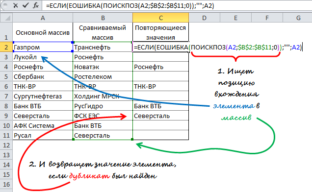
In cell C2, enter the following formula \u003d IF (ISERROR (SEARCH (A2; $ B $ 2: $ B $ 11; 0)); ""; A2) and extend it to cell C11. This formula sequentially searches for each item from column A in column B and returns the item's value if found in column B.
Using the VLOOKUP substitution formula
The principle of the formula is similar to the previous method, the difference lies in, instead of SEARCH. Distinctive feature This method is also the ability to compare two horizontal arrays using the HLP formula.
To compare two columns with the data in columns A and B (similar to the previous method), enter the following formula \u003d VLOOKUP (A2; $ B $ 2: $ B $ 11; 1; 0) into cell C2 and drag it to cell C11.
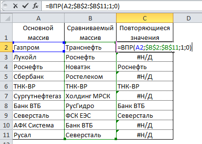
This formula looks at each element from the main array in the compared array and returns its value if it was found in column B. Otherwise, Excel will return a # N / A error.
Using VBA Macro
Using macros to compare two columns can unify the process and reduce data preparation time. The decision about which comparison result should be displayed depends entirely on your imagination and skills in using macros. Below is the technique published on the official Microsoft website.
1 | Sub Find_Matches () |
In this code, the CompareRange variable is assigned the range with the compared array. It then runs a loop that loops through each item in the selected range and compares it to each item in the range being compared. If elements with the same values \u200b\u200bwere found, the macro enters the value of the element in column C.
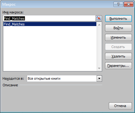
To use the macro, return to the worksheet, select the main range (in our case, these are cells A1: A11), press Alt + F8. In the dialog that appears, select the macro Find_Matchesand click the execute button.
After executing the macro, the result should be as follows:
![]()
Using the Inquire add-in
Outcome
So, we looked at several ways to compare data in Excel that will help you solve some analytical problems and make it easier to find duplicate (or unique) values.
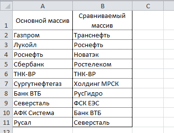
We have two tables of orders copied into one worksheet. It is necessary to compare the data of two tables in Excel and check which positions are in the first table, but not in the second. There is no point in manually comparing the value of each cell.
Compare two columns for matches in Excel
How to make comparison of values \u200b\u200bin Excel of two columns? To solve this problem, we recommend using conditional formatting, which can quickly highlight the items that are in only one column in color. Worksheet with tables:
The first step is to assign names to both tables. This makes it easier to understand which cell ranges are being compared:
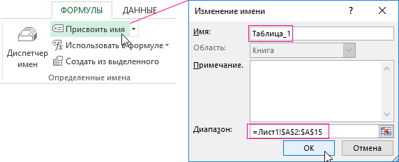
- Select the FORMULAS tool - Defined Names - Assign Name.
- In the window that appears, in the "Name:" field, enter the value - Table_1.
- Left-click on the "Range:" entry field and select the range: A2: A15. And click OK.
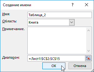
For the second list, do the same, but assign a name - Table_2. And indicate the range C2: C15 - respectively.
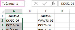
Helpful advice! Range names can be assigned more quickly by using the name field. It is located to the left of the formula bar. Just select the ranges of cells, and in the name field, type the appropriate name for the range and press Enter.
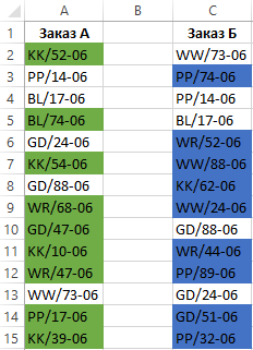
Now let's use conditional formatting to compare two lists in Excel. We need to get the following result:
Positions that are in Table_1, but not in Table_2 will be displayed in green... At the same time, the positions located in Table_2, but absent in Table_1, will be highlighted in blue.

Principle of comparing data of two columns in Excel
We used the COUNTIF function to define the conditions for formatting the column cells. In this example, this function checks how many times the value of the second argument (for example, A2) occurs in the list of the first argument (for example, Table_2). If the number of times \u003d 0 then the formula returns TRUE. In this case, the cell is assigned the custom format specified in the conditional formatting options. The reference in the second argument is relative, which means that all cells of the selected range will be checked in turn (for example, A2: A15). The second formula works in a similar way. The same principle can be applied to various similar tasks. For example, to compare two prices in Excel, even