Different tables in excel samples
If you've never used a spreadsheet to create documents before, we recommend reading our Excel guide for dummies.
Then you can create your first spreadsheet with tables, graphs, math formulas and formatting.
Detailed information on basic functions and capabilities table processor ... Description of the main elements of the document and instructions for working with them in our material.
By the way, to work more effectively with Excel tables, you can familiarize yourself with our material.
Working with cells. Padding and formatting
Before proceeding with specific actions, you need to understand basic element anyone. An Excel file consists of one or more sheets divided into small cells.
A cell is a basic component of any Excel report, spreadsheet or graph. Each cell contains one block of information. It can be a number, date, currency, unit of measure, or other data format.
To fill in a cell, just click on it with the pointer and enter the required information. To edit a previously filled cell, double-click on it.

Figure: 1 - an example of filling cells
Each cell on the sheet has its own unique address. Thus, you can carry out calculations or other operations with it. When you click on a cell, a field with its address, name and formula will appear at the top of the window (if the cell is involved in any calculations).
Let's select the cell "Share of shares". Its location address is A3. This information is indicated in the properties panel that opens. We can also see the content. This cell has no formulas, so they are not shown.
More cell properties and functions that can be used in relation to it are available in the context menu. Click on the cell with the right key of the manipulator. A menu will open with which you can format the cell, analyze the content, assign a different value, and other actions.

Figure: 2 - context menu of a cell and its main properties
Sorting data
Often users are faced with the task of sorting data on a sheet in Excel. This feature helps you quickly select and view only the data you want from the entire table.
Before you already (we will figure out how to create it later in the article). Imagine that you want to sort the data for January in ascending order. How would you do it? A banal retyping of a table is an extra work, besides, if it is voluminous, no one will do it.
Excel has a special function for sorting. The user is only required to:
- Select a table or block of information;
- Open the "Data" tab;
- Click on the "Sort" icon;
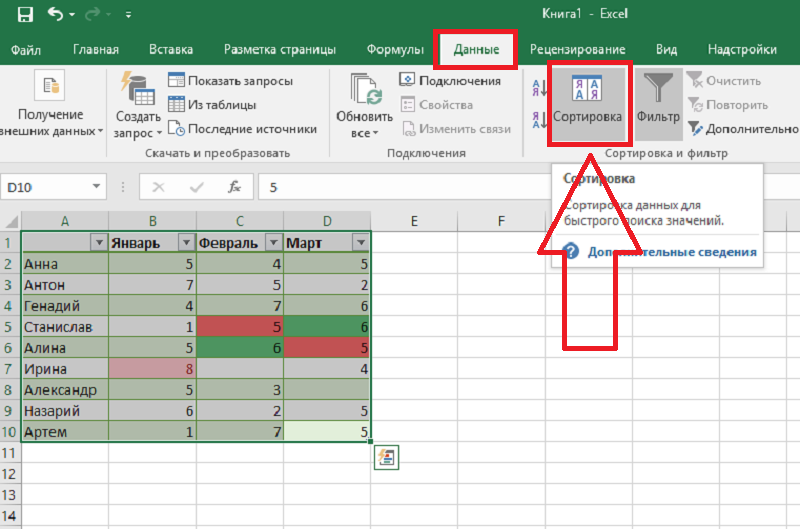
Figure: 3 - "Data" tab
- In the window that opens, select the column of the table, over which we will carry out actions (January).
- Next, the sorting type (we are grouping by value) and, finally, the order is ascending.
- Confirm the action by clicking on "OK".
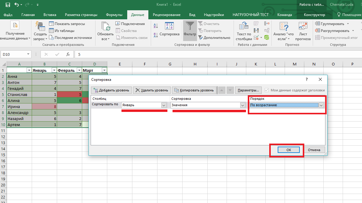
Figure: 4 - setting sorting parameters
The data will be automatically sorted:
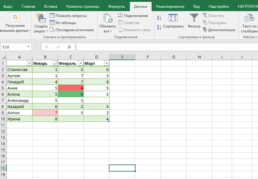
Figure: 5 - the result of sorting the digits in the column "January"
Similarly, you can sort by color, font and other parameters.
Mathematical calculations
The main advantage of Excel is the ability to automatically carry out calculations in the process of filling out the table. For example, we have two cells with values \u200b\u200b2 and 17. How can we enter their result into the third cell without doing the calculations ourselves?
To do this, you need to click on the third cell in which the final result of the calculations will be entered. Then click on the function icon f (x) as shown in the figure below. In the window that opens, select the action you want to apply. SUM is the sum, AVERAGE is the average, and so on. Full list functions and their names in the Excel editor can be found on the official website of Microsoft.
We need to find the sum of two cells, so we click on "SUM".
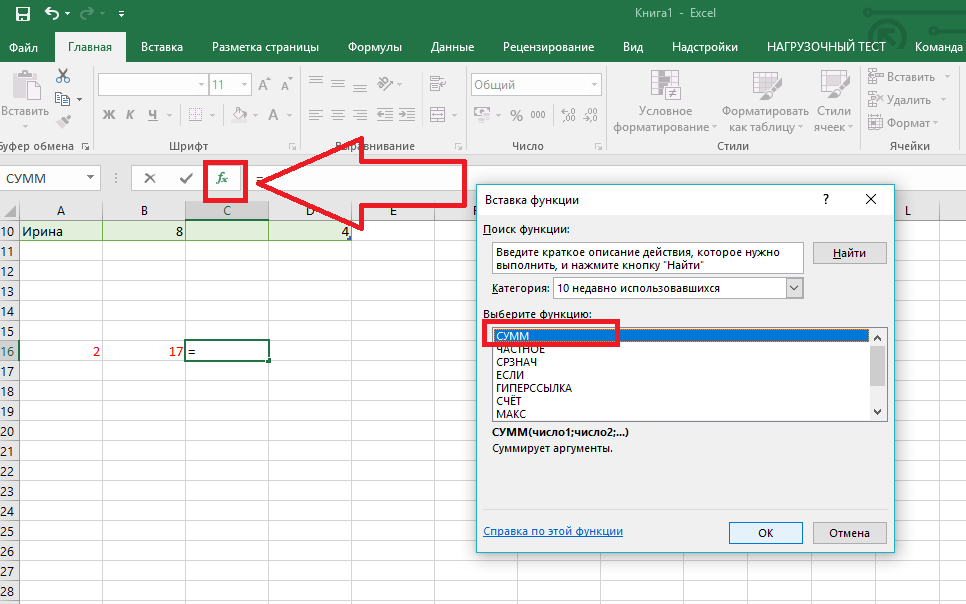
Figure: 6 - selection of the "SUM" function
There are two fields in the function arguments window: "Number 1" and "Number 2". Select the first field and click on the cell with the number "2". Its address will be written to the argument string. Click on "Number 2" and click on the cell with the number "17". Then confirm the action and close the window. If you need to perform math with three or more boxes, just keep entering the argument values \u200b\u200bin the Number 3, Number 4, and so on.
If the value of the summed cells changes in the future, their sum will be updated automatically.
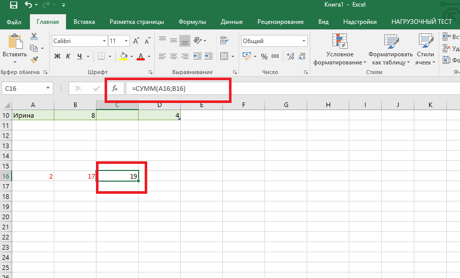
Figure: 7 - the result of the calculations
Creating tables
Any data can be stored in Excel tables. With the help of the quick setup and formatting function, it is very easy in the editor to organize a personal budget control system, a list of expenses, digital data for reporting, and more.
They have an advantage over a similar option in other office programs. Here you have the opportunity to create a table of any dimension. The data is filled in easily. There is a function panel for editing content. In addition, ready table can be integrated into a docx file using the usual copy-paste function.
To create a table, follow the instructions:
- Click the Insert tab. On the left side of the options pane, select Table. If you need to carry out the mixing of any data, select the item " Pivot table»;
- Using the mouse, select a place on the sheet that will be allocated for the table. And also you can enter data location in the element creation window;
- Click OK to confirm the action.

Figure: 8 - creating a standard table
To format appearance of the resulting plate, open the contents of the constructor and in the "Style" field click on the template you like. If desired, you can create your own look with a different color scheme and cell selection.

Figure: 9 - table formatting
The result of filling the table with data:

Figure: 10 - filled table
For each cell in the table, you can also customize the data type, formatting and information display mode. The designer window contains all the necessary options for further configuration of the plate, based on your requirements.
Data grouping
When you're preparing a priced product catalog, it's a good idea to think about usability. A large number of positions on one sheet forces you to use search, but what if the user only makes a choice and has no idea about the name? In Internet catalogs, the problem is solved by creating product groups. So why not do the same in an Excel workbook?
Grouping is easy enough. Select several lines and press the button Group in the tab Data (see fig. 1).
Figure 1 - Grouping button
Then specify the type of grouping - line by line (see fig. 2).

Figure 2 - Selecting the type of grouping
As a result, we get ... not what we need. The product lines have been combined into a group indicated below them (see Fig. 3). Directories usually have the header first and then the content.

Figure 3 - Grouping rows "down"
This is not a software bug. Apparently, the developers thought that the grouping of lines is mainly done by the compilers of financial statements, where the final result is displayed at the end of the block.
To group rows up, you need to change one setting. In the tab Data click on the small arrow in the lower right corner of the section Structure (see fig. 4).
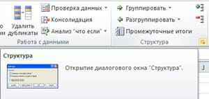
Figure 4 - The button responsible for displaying the structure settings window
In the settings window that opens, uncheck the box Totals in rows below data(see fig. 5) and press the button OK.

Figure 5 - Structure settings window
All groups that you managed to create will automatically change to the "top" type. Of course set parameter will also affect the further behavior of the program. However, you will have to uncheck this box to each new sheet and every new Excel workbook, because the developers did not provide for a "global" setting of the grouping type. Likewise, you cannot use different types of groups within the same page.
Once you have categorized the products, you can collect the categories into larger sections. In total, there are up to nine levels of grouping.
The inconvenience when using this function is the need to press the button OK in the pop-up window, and it will not be possible to collect unrelated ranges in one go.

Figure 6 - Multilevel directory structure in Excel
Now you can expand and close parts of the catalog by clicking on the pluses and minuses in the left column (see Fig. 6). To expand the entire level, click on one of the numbers at the top.
To bring rows to a higher level in the hierarchy, use the button Ungroup tabs Data... You can completely get rid of the grouping using the menu item Delete structure (see fig. 7). Be careful, it is impossible to undo the action!
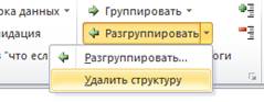
Figure 7 - Remove row grouping
Freezing sheet regions
Quite often, when working with Excel tables, it becomes necessary to freeze some areas of the sheet. This may include, for example, row / column headings, company logo or other information.
If you freeze the first row or the first column, then everything is very simple. Open the tab View and in the dropdown menu To fix areas select items accordingly Pin top line or Freeze first column (see fig. 8). However, it will not be possible to “freeze” both the row and the column in this way.
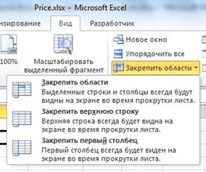
Figure 8 - Fixing a row or column
To unpin, select the item in the same menu Unpin regions (clause replaces the string To fix areasif the page is frozen).
But pinning multiple rows or an area of \u200b\u200brows and columns is not so transparent. You select three lines, click on the item To fix areas, and ... Excel only "freezes" two. Why is that? An even worse option is possible, when the areas are fixed in an unpredictable way (for example, you select two lines, and the program puts the borders after the fifteenth). But let's not write it off as an oversight of the developers, because the only correct use of this function looks different.
You need to click on the cell below the rows that you want to freeze, and, accordingly, to the right of the docked columns, and only then select the item To fix areas... Example: in Figure 9, a cell is selected B 4... This means that three rows and the first column will be fixed, which will remain in their places when scrolling the sheet both horizontally and vertically.

Figure 9 - Fix the area of \u200b\u200brows and columns
You can apply a background fill to the docked areas to indicate to the user special behavior of these cells.
Rotate the sheet (replace rows with columns and vice versa)
Imagine this situation: you worked for several hours on a set of spreadsheets in Excel and suddenly realized that you did not design the structure correctly - the column headings should have been painted by row or row by column (it does not matter). Do you want to retype everything manually? Never! Excel provides a function that allows you to "rotate" the sheet 90 degrees, thus moving the contents of the rows into columns.
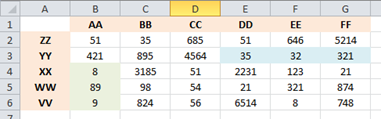
Figure 10 - Source table
So, we have some table that needs to be "rotated" (see Fig. 10).
- Select cells with data. It is the cells that are highlighted, not the rows and columns, otherwise nothing will work.
- Copy them to the clipboard with a keyboard shortcut
or in any other way. - Go to an empty sheet or free space of the current sheet. Important note: cannot be inserted over the current data!
- Insert data with a keyboard shortcut
and in the insert options menu, select the option Transpose (see fig. 11). Alternatively, you can use the menu Paste from tab the main (see fig. 12).
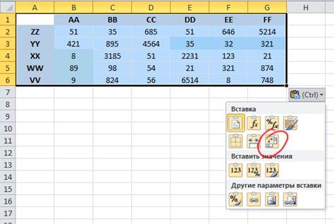
Figure 11 - Insert with transposition
![]()
Figure 12 - Transpose from the main menu
That's all, the table has been rotated (see Fig. 13). In this case, the formatting is preserved, and the formulas are changed in accordance with the new position of the cells - no routine work is required.
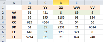
Figure 13 - Result after rotation
Show formulas
Sometimes a situation arises when you cannot find the required formula among a large number of cells, or you simply do not know what and where to look for. In this case, the ability to display not the result of calculations, but the original formulas will be useful to you.
Click the button Show formulas in the tab Formulas (see Figure 14) to change the presentation of the data in the worksheet (see Figure 15).

Figure 14 - "Show formulas" button
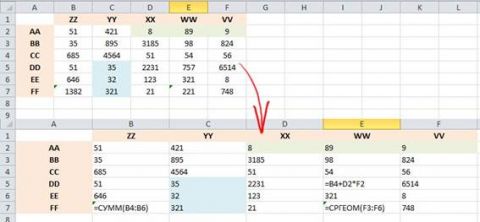
Figure 15 - Formulas are now visible on the sheet, and not the results of the calculation
If you find it difficult to navigate the cell addresses displayed in the formula bar, click Influence cells from tab Formulas (see fig. 14). Dependencies will be shown with arrows (see Fig. 16). To use this feature, you must first highlight one cell.

Figure 16 - Cell dependencies are shown by arrows
Hiding dependencies at the click of a button Remove arrows.
Wrap lines in cells
Quite often in Excel workbooks there are long labels that do not fit in the cell in width (see Fig. 17). You can, of course, push the column apart, but this option is not always acceptable.
Figure 17 - Labels do not fit into cells
Select cells with long labels and press the button Wrap text on The main tab (see fig. 18) to switch to multi-line display (see fig. 19).
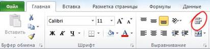
Figure 18 - Button "Text wrapping"

Figure 19 - Multi-line display of text
Rotate text in a cell
Surely you have come across a situation where the text in the cells needed to be placed not horizontally, but vertically. For example, to label a group of rows or narrow columns. Excel 2010 provides tools to rotate text in cells.
Depending on your preference, you can go in two ways:
- First create the label, and then rotate it.
- Adjust the rotation of the label in the cell, and then enter the text.
The options differ slightly, so we will consider only one of them. To begin with, I concatenated six lines into one using the button Merge and center on The main tab (see fig. 20) and entered a generalizing inscription (see fig. 21).
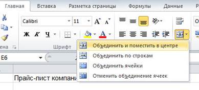
Figure 20 - Button for merging cells
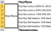
Figure 21 - First, create a horizontal signature
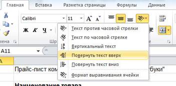
Figure 22 - Text rotation button
You can further reduce the column width (see Figure 23). Done!
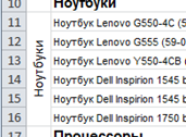
Figure 23 - Vertical cell text
If you wish, you can set the text rotation angle manually. In the same list (see Figure 22), select Cell alignment format and in the window that opens, specify an arbitrary angle and alignment (see Fig. 24).
Figure 24 - We set an arbitrary angle of rotation of the text
Conditionally formatting cells
Opportunities conditional formatting appeared in Excel for a long time, but by the 2010 version they were significantly improved. You may not even have to understand the intricacies of creating rules, because the developers have provided for many blanks. Let's take a look at how to use conditional formatting in Excel 2010.
The first thing to do is select the cells. Further on The main tab click Conditional formatting and select one of the blanks (see fig. 25). The result will be displayed on the sheet immediately, so you don't have to go through the options for a long time.
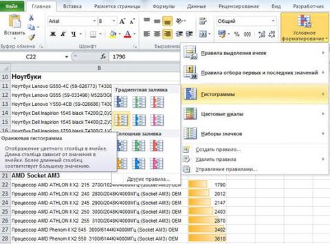
Figure 25 - Selecting a preset conditional formatting
The histograms look quite interesting and reflect well the essence of price information - the higher it is, the longer the segment.
Color bars and icon sets can be used to indicate various states, such as transitions from critical costs to acceptable costs (see Figure 26).
Figure 26 - Color scale from red to green with intermediate yellow
You can combine histograms, scales, and icons in the same range of cells. For example, the bar graphs and icons in Figure 27 show acceptable and excessively low device performance.
Figure 27 - The histogram and set of icons reflect the performance of some conventional devices
To remove conditional formatting from cells, select them and from the conditional formatting menu, choose Remove rules from selected cells (see fig. 28).

Figure 28 - Removing the Conditional Formatting Rules
Excel 2010 uses presets to quickly access conditional formatting capabilities. customizing your own rules is far from obvious to most people. However, if the templates provided by the developers do not suit you, you can create your own rules for the design of cells according to various conditions. Full description this functionality is beyond the scope of the current article.
Using filters
Filters allow you to quickly find the information you need in a large table and present it in a compact form. For example, from a long list of books you can choose works by Gogol, and from the price list of a computer store - Intel processors.
Like most other operations, the filter requires selection of cells. However, you do not need to select the entire table with data; it is enough to mark the rows above the required data columns. This greatly increases the usability of the filters.
After the cells are selected, in the tab the main press the button Sort and filter and select item Filter (see fig. 29).
Figure 29 - Create filters
The cells will now turn into drop-down lists where you can set the selection parameters. For example, we look for all references to Intel in the column Name of product... To do this, select the text filter Contains (see fig. 30).
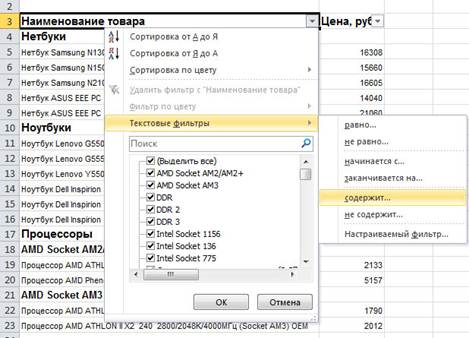
Figure 30 - Create a text filter
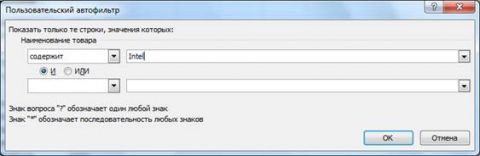
Figure 31 - Create a filter by word
However, it is much faster to achieve the same effect by writing a word in the field Search the context menu shown in Figure 30. Why then call an additional window? It is useful if you want to specify multiple selection conditions or select other filtering options ( does not contain, starts with ..., ends with ...).
For numeric data, other parameters are available (see Figure 32). For example, you can select 10 largest or 7 smallest (the number is configurable).

Figure 32 - Numeric filters
Excel filters provide a fairly rich feature comparable to the SELECT query in database management systems (DBMS).
Displaying information curves
Information Curves (Sparklines) are an innovation in Excel 2010. This feature allows you to display the dynamics of changes in numeric parameters directly in a cell, without having to build a chart. Changes in numbers will be immediately shown on the micrograph.
Figure 33 - Excel 2010 Sparkline
To create a sparkline, click on one of the buttons in the block Infocurves in the tab Insert (see Figure 34), and then set the range of cells to build.
Figure 34 - Inserting a hot curve
Like charts, information curves have many options to customize. More detailed manual how to use this functionality is described in the article.
Conclusion
This article covered some useful Excel 2010 features that can speed up your work, improve the look of your tables, or improve usability. It doesn't matter if you create the file yourself or use someone else's - Excel 2010 has functions for all users.
Hello, in this tutorial you will learn the basics of working with spreadsheets in Excel. You will learn about rows, columns, cells, worksheets and books in Excel. I will tell you everything you need to know to get started with MS Excel. Let's get started.
Basic concepts
Rows - rows in Excel are numbered starting from 1. The cells in the first row will be A1, B1, C1, and so on.
Columns - columns in Excel are denoted by Latin letters starting with A. The cells in the first column will be A1, A2, A3 and so on.
The selected cell displays which table cell you are currently working with.
A cell reference shows the address of the selected cell.
The formula bar displays information entered in the selected cell, be it a number, text, or a formula.
How to select a cell
There are several ways to select a cell:
- To select one cell, just click on it with the left mouse button
- To select the entire line, click on the line number
- To select an entire column, click on the letter of the column
- To select several adjacent cells, click on a corner cell, hold down the left mouse button and drag left / right, up / down.
- To select several non-adjacent cells, click on them while holding down Ctrl.
- To select each cell on the sheet, click in the upper right corner of the sheet to the left of "A"
In order to enter data in any cell, select it by clicking on it with the left mouse button, and then type the information you need using the keyboard. When you enter data, it also appears in the formula bar.
How to edit the contents of a cell.
In order to change the contents of a cell in Excel, select it by double-clicking the left mouse button. Or select by standard method and then press F2. Also you can change data in cells using in the formula bar.
How to move between cells using the keyboard
Use the arrow keys to move between cells in excel spreadsheets... Press Enter to move one cell down, or Tab to move one cell to the right.
How to move or copy a cell
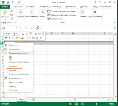
In order to copy the cell data, first click on it with the right mouse button and select "Copy", then right-click again, but on the cell where you want to paste the information and select Paste Options: Paste.
To move a cell, right-click on it and select Cut, then in the desired cell, right-click again and select Paste.

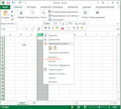
How to insert a column or row
In order to insert a column in Excel, right-click on the letter of the column and select Insert. Excel always inserts the column to the left of the selected column.
To insert a row into Excel, right-click on the row number and select Insert. Excel always inserts a row above the selected row.
Summary
Today you learned about the basic methods of working in Excel, such as selecting, copying and moving cells, inserting columns and rows, entering and changing data in cells.
If you have any questions, ask them in the comments below the article.