How to make a spreadsheet in Excel. Training to work in excel.
Hi everyone! Today's material for those who continue to master the work with application programs, and do not know how to do pivot table in excel.
Having created a general table, in any of text documents, you can analyze it by doing in Excel pivot tables.
Creating a pivot Excel table requires certain conditions to be met:
- The data fits into a table with columns and lists with names.
- Lack of blank forms.
- Lack of hidden objects.
How to make a pivot table in excel: step by step instructions
To create a pivot table, you must:

A blank sheet has been created, where you can see the lists of areas and fields. The headings have become fields in our new table. The pivot table will be formed by dragging and dropping fields.
They will be marked with a tick, and for the convenience of analysis, you will swap them in the table areas. 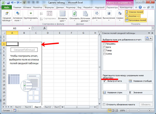
I decided that I would analyze the data through a filter by sellers, so that it would be visible by whom and for how much each month was sold, and what kind of product.
We select a specific seller. Click the mouse and drag the field "Salesperson" to the "Report filter". The new field is ticked and the table view changes slightly. 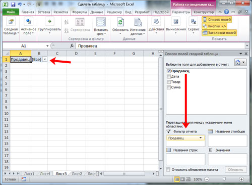
We will put the category "Products" in the form of strings. We transfer the required field to "Line names". 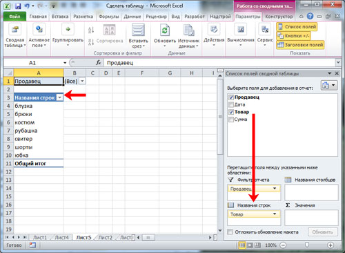
To display the drop-down list, it matters in which order we specify the name. If initially we make a choice in favor of the product in the lines, and then we indicate the price, then the products will be the drop-down lists, and vice versa.
The "Units" column, being in the main table, displayed the quantity of goods sold by a specific seller at a specific price. 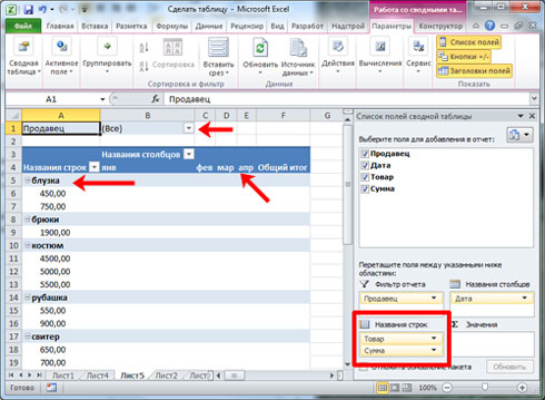
To display sales, for example, for each month, you need to replace the “Date” field with the “Column names”. Select the "Group" command by clicking on the date. ![]()
We indicate the periods of the date and the step. We confirm the choice. 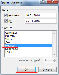
We see such a table. 
Let's transfer the "Amount" field to the "Values" area. 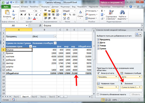
The display of numbers became visible, but we need exactly the number format 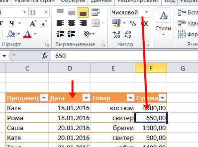
To fix it, select the cells, call the window with the mouse, select "Number format".
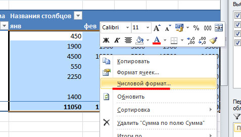
We choose the number format for the next window and mark the "Group separator". Confirm with the "OK" button. 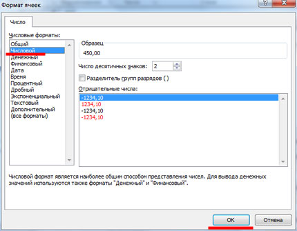
Pivot table design
If we check the box that confirms the selection of several objects at once, then we will be able to process data for several sellers at once. 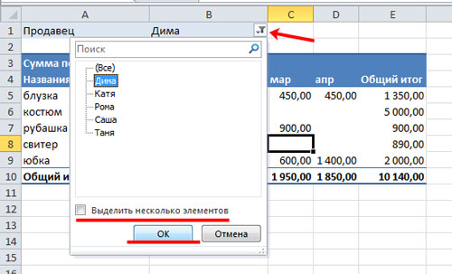
The filter can be applied to columns and rows. By checking the box on one of the product types, you can find out how much of it has been sold by one or more sellers. 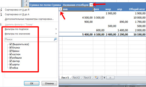
The field parameters are also configured separately. In the example, we see that a certain Roma seller sold shirts for a specific amount in a specific month. By clicking the mouse, we call the menu in the line "Sum by field ..." and select "Parameters of value fields". 
Next, for data reduction in the field, select "Quantity". We confirm the choice. 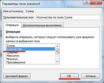
Take a look at the table. It clearly shows that in one of the months the seller sold 2 shirts. 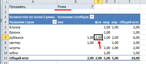
Now we change the table and make the filter work by months. We move the field "Date" to the "Report filter", and where the "Column names" will be "Seller". The table displays the entire sales period or for a specific month.

Selecting cells in a PivotTable will bring up a tab such as PivotTable Tools, and there will be two more tabs, Options and Design. 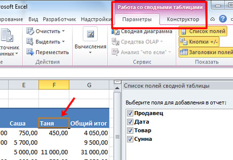
In fact, you can still talk about the settings of pivot tables for a very long time. Make changes to your taste, achieving a convenient use for you. Feel free to push and experiment. You can always change any action by pressing the Ctrl + Z keyboard shortcut.
I hope you have mastered all the material and now you know how to make a pivot table in excel.
Creating tables in special programs, text or graphic editors, greatly simplifies the perception of text that has any numerical data. And each program has its own characteristics. In this article, we will consider how to make a table in Excel.
Essentially, Excel worksheet is initially presented in the form of a table. It consists of a large number of cells, which have their own specific address - the name of the column and the row for this cell. For example, let's select any cell, it is in column B, in the fourth row - address B4. It is also listed in the Name field.
When printing Excel worksheets with data, neither cell borders nor row and column names will be printed. This is why it makes sense to figure it out how to create a table in Excel so that the data in it is limited and separated... In the future, it can be used for and for according to the available data.
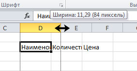
Let's start by creating a header for the table. Enter the desired names in the cells. If it does not fit, the cells can be expanded: move the cursor to the column name, it will take the form of a black arrow pointing in different directions, move it to the required distance.
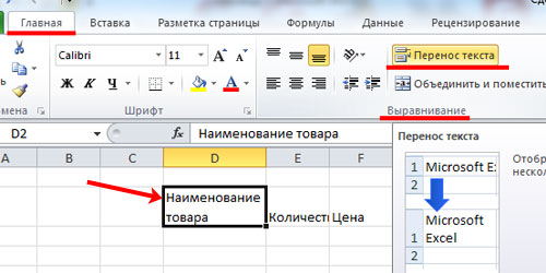
Another way to place text in a cell is to wrap it. Select the cell with the text and on the "Home" tab in the "Alignment" group click on the button "Text wrapping".
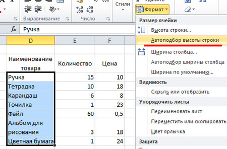
Now let's fill the table with the required data. In cell D8, I used the text wrapping, let's make it visible in full and the cells are the same height. Select the cells in the required column, and on the "Home" tab in the "Cells" group, click on the "Format" button. Select "Row Height" from the list.
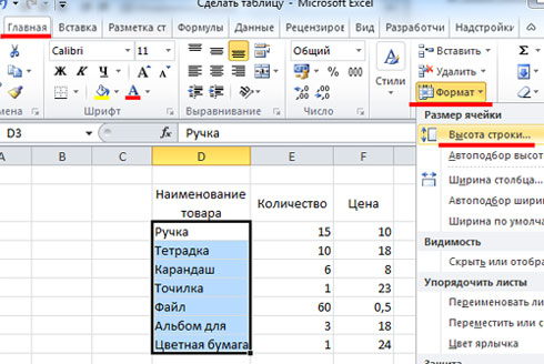
Enter a suitable value in the dialog box. If it is not necessary that the lines be the same height, you can click on the button "Auto-fit line height".
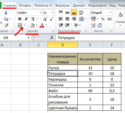
On the "Home" tab, in the "Font" and "Alignment" groups, you will find buttons for formatting the table. There will also be a button for creating borders. Select a range of table cells, click on the black arrow next to the button and select "All Borders" from the list.
That's how quickly we made a table in Excel.
You can also create a table in Excel using the built-in editor.... In this case, she will be called smart table.
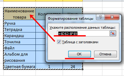
Let's select our entire table along with the header and data. Then on the "Home" tab in the "Styles" group click on the button "Format as Table"... Select the appropriate style from the list.

A dialog box appears indicating the range of cells for the table. Check the box "Table with headers"... Click OK.
The table will appear in accordance with the selected style. This did not happen for me, because before that I formatted the selected range of cells.
Now I will remove the borders and fill for the column names - those parameters that I selected earlier. This will display the selected style.
If you remember, we made a smart table in Excel... To add a new column or row, start entering data into any cell that is adjacent to the table and press "Enter" - it will automatically expand.
When you select a table, a new tab appears on the ribbon "Working with tables" - "Constructor". Here you can set the desired name for the table, make a pivot table, add a total row to the table, highlight rows and columns, change the style.

Smart excel tables good to use for, various other charts and for. Since when new data is added to it, they are immediately displayed, for example, in the form of building a new graph on a diagram.
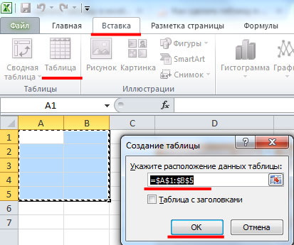
You can create a smart table in another way. Select the required range of cells, go to the "Insert" tab and click on the "Table" button. In the dialog box that appears, the selected range will be indicated, check the box "Table with headers" and click OK.
So, in just a couple of clicks, you can make a regular or smart table in Excel.
I showed and told what it is, its main functions. Now let's get down to the practical application of this knowledge.
Excel tables will become your irreplaceable helpers in everyday life and in business.
If you came to the Internet to make money, you should know that your business will help you. But you should have and how to come to it.
The Excel spreadsheet editor will become a tool with which you can calculate your costs and income. You will clearly see the amount of money received from the projects you have chosen. You will be able to calculate in advance how much income you will get within the timeframe you have planned.
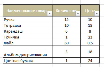
The first thing to write is column names:
- name
- amount
- sum
Then list purchases:
- Butter
- Sugar
At the end of the first column, write “Total”. Indicate the price and quantity of the purchased products. To move from one cell to another, use the "Enter" key.
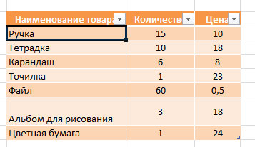
You can increase the size of the font, change its color and theme. It is possible to change the colors of the cells. If the name of the cell does not fit, then in this case, go to the name of the column, put the cursor on the border of the columns and drag to the right to the size we need.
We define the boundaries of your table. To do this, select the plate by holding the left mouse and stretching it from the upper left corner to the lower right. Go to the "Home" tab and click on "Borders". In the drop-down submenu, select "All borders".
After that, you can choose the color of the plate, its individual lines. Do everything according to your taste: beautiful and comfortable.
We can say that the plate for calculating the costs of purchases is ready.
Now get started to calculations... It is necessary to perform an action - multiplying the price by the quantity. Place the cursor in column "D" in the line "Bread" and type from the keyboard: "\u003d". Then click on the quantity of this product - column "B". From the keyboard, click on the multiplication sign: "*" (Do not forget to hold the "Shift" button at the same time) and click in the "C" column on the price of this product. Then press "Enter".
Next, we'll use the autocomplete marker. We bring the cursor to the lower right border of the cell with the amount calculated by you and, clamping the corner, pull it down. The cells will copy the formulas, as it were, and the calculation will be performed immediately. You no longer have to do it manually.
 Now it remains to calculate the auto-sum. Select the cells in the "D" column. Go to the "Home" tab and select the "Σ" icon.
That's it, the total purchase costs have been calculated!
What else can you change in your nameplate?
When you write numbers in cells, they can be in the format of a date, general, monetary, percentage. To set the format, select the numbers and in the "Home" tab go to "General" and select whatever you need. Capture only numbers when selecting. No words needed.
You can use the function of combining cells. For example, for the title of a table. Swipe from the beginning of the header line to the end of the table. Go to the "Home" tab - "Align" group - "merge and place in the center". Then use the buttons for the location of the text, as in the Word, and select the font size.
 Let's format the object. To do this, you need to select the plate without a title. Then go to the "Insert" tab. Choose: "Table". Recheck all your titles and titles. In the drop-down menu, click "OK".
Now you have each column name contains the "Filter" function. By applying a filter to a name, one or another row of the table can be considered separately. This helps to single out one or several items from a large number of items and consider only them.
In order to remove the filter from each of the columns, in the "Home" tab, click on "Sort and Filter" - "Filter". The reverse operation can be done in the same way.
The "Constructor" function appears in the "Menu" line. With its help, it is possible to change the styles of the table.
If you want to add additional rows or columns, right-click on the existing one and select "Insert".
If you want to change the inscription in the cell, click inside 2 times and write a new name or number. To delete the contents of a cell - select it and press the "Del" key.
Congratulations!
Now you have a full-fledged excel spreadsheet... You did it! A start! Now Excel spreadsheet editor in your hands.
To save your masterpiece, click in the upper left corner on the quick access panel "Save".
And now I propose to see this Video... It shows and tells more clearly and in detail how create a table in Excel:
Summarize. It's easy and simple to create a spreadsheet in Excel. You just have to want it. The Excel spreadsheet editor can become your indispensable assistant in calculating income, expenses, profits in certain companies, forecasts and winnings.
And I wish you all the best and look forward to your comments.
With love and gratitude , Svetlana Duban - Aurora
My skype: aleksandra200628
The fact that the ability to work on a computer today is necessary for everyone and everyone does not raise doubts even among skeptics.
The book you are holding in your hands will be a real friend and helper for those who wish to independently and in a short time master the wisdom of working on personal computer... Written in a simple and straightforward language, it is accessible and easy even for beginners. A large number of specific examples and illustrative illustrations contributes to the quick and easy assimilation of the proposed material.
Its sequential presentation, as well as a detailed step-by-step description of the key operations and procedures, make the study of this book a fascinating process, the result of which will be the ability to communicate "well" with any modern computer.
The description is based on the example of Windows XP Professional.
Book:
As we noted above, the worker excel sheet is a table consisting of cells, each of which is formed as a result of the intersection of a row and a column. But after all, the worksheet is almost never completely filled with data: it usually contains small tables. Accordingly, they need to be somehow indicated on the sheet, having appropriately formalized the visual presentation of a specific table. In particular, the rows and columns of the table should have clear names that reflect their essence, the table should have clear boundaries, etc.
To solve this problem, a special mechanism is implemented in Excel, which is accessed using the toolbar. Boundaries... You can enable the display of this panel (Fig. 6.21) using the command of the main menu View? Toolbars? Border.
Fig. 6.21. Toolbar Border
First you have to decide what border you want to draw. For example, the common border of the table can be highlighted with bold lines, and the grid of the table - with regular lines, etc. To draw a common border, you need to click the button located on the left in the toolbar, and in the menu that opens (see Fig. 6.21) select the item Picture border... Then, while holding down the mouse button, use the pointer (which will take the shape of a pencil) to outline the border of the table. In order for each cell to be separated from one another by a border, you need to select the item in the menu (see Fig. 6.21) Boundary grid, after which, while holding down the mouse button, draw a range, the cells of which should be separated by a border.
* * *
In fig. 6.22 shows an example of a table created using three types of lines: bold, dash-dotted and double.
![]()
Fig. 6.22. Table design option
But that's not all: if you wish, you can decorate each line with any color. To select a color, click in the panel Boundariesthe last button on the right, and specify it in the menu that opens.
Please note that the table borders created in this way cannot be deleted by the traditional method - by pressing the key Delete... To do this, you need in the panel Borderpush the button Erase the border(its name is displayed as a tooltip when you hover the mouse pointer), then perform the same actions as in the process of creating a border (i.e., while holding down the mouse button, specify the lines to be erased). To delete a line within one cell, it is enough to move the mouse pointer to this line, which after pressing the button Erase the borderwill take the form of an eraser, and just click
However, drawing a table is only half the battle: to perform interactive calculations in it, you need to create formulas or apply the appropriate functions. We will consider these operations below, using a specific example.
The easiest thing to do in Microsoft Excel - create a table. Consider this process at microsoft example Office 2007.
The first thing to start with is to calculate the required number of columns and rows. Let's say we need 5 columns and 6 rows. Accordingly, we highlight columns A-E and lines 1-6. 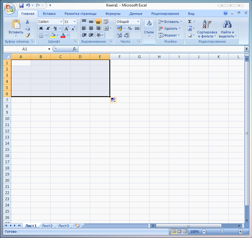
This option is suitable if you need to create an empty table in which data can be entered after creating or after printing the table. Or, you can immediately fill in the required number of columns and rows with data, after which all that remains is to frame the table. We will focus on creating an empty table.
Select, click on the selected area with the right mouse button and select Cell format.
![]()
In the window that opens, go to the tab Border... This setting is responsible for how the separators will look in the table. Accordingly, you can configure appearance tables as desired. But we will not come up with something sophisticated for an example, but we will create a classic table. 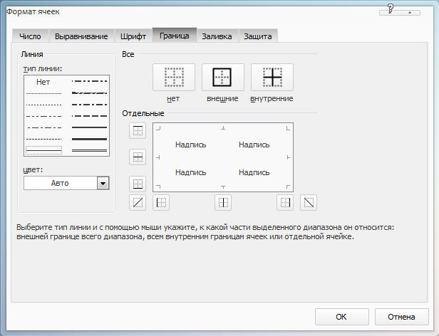
For this we choose Line type bold (the boldst stripe), in the section All choose External... This is how we created the outer borders of the table, the inner separators can be made immediately, for this in Line type choose the usual lane, in the section All choose Internal. Color you can leave Auto - by default it is black. Now you can click OK... The result will be like this: 
If you want to make the inner dividers as bold as the outer frame, then reopen the tab Border, in section All choose Internal, Line type choose bold.
It is worth noting that you must first select the line type and then the border type, and not vice versa.
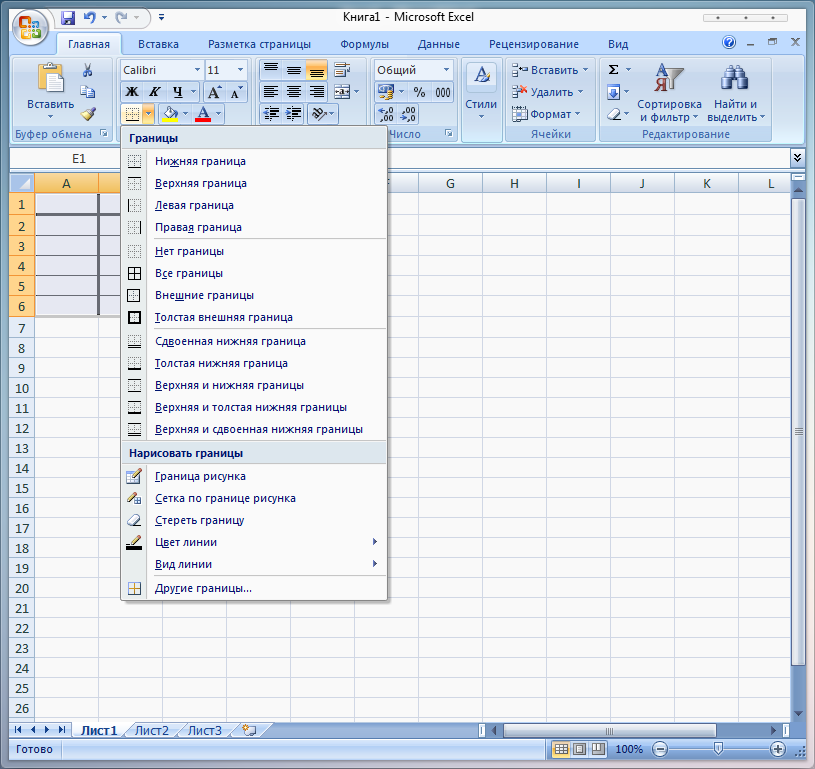
Often times, the first line in a table has a bold border that separates it from the rest of the lines. To do this, select the entire first line, open the tab Border, Line type choose bold, in the section All choose External... The same can be done with the first column. The result will be like this: 
You can also customize the borders at your discretion through the top toolbar:
You can adjust the width of columns or rows by hovering over the letter or number separators. 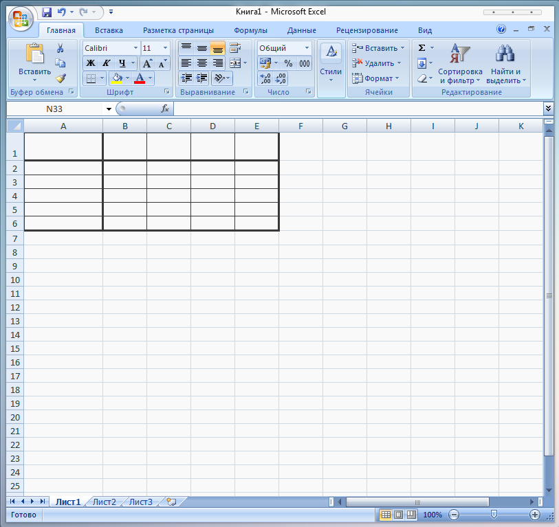
If you need to fill a column or row with color, then select the area, right-click and select Cell format... In the window that opens, select the tab Fill and choose the desired color. The result will be something like this: 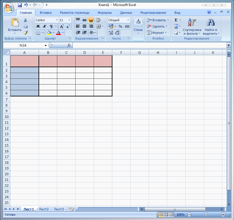
Done! The resulting table can now be filled in, saved or printed.