How to calculate the amount of a column in Excel. How to calculate the sum of a column in Excel. How to calculate the amount in a column using the AutoSum button

Perhaps one of the most popular features microsoft programs Excel is addition. Excel's simplicity of summing values \u200b\u200bmakes a calculator or other ways of adding large arrays of values \u200b\u200balmost useless. An important feature of addition in Excel is that the program provides several ways to do this.

It is recommended that a report on pivot table was created in a new table. Click the Accept button to complete the dynamic table creation. It has three components. These are the column headings that contain the qualitative or quantitative data that make up the database.

Sum of values \u200b\u200bfor information

Here you drag and drop the fields and depending on your position from 4 possible areas, this will be a summary of the observed information. In this section, the result of the information is observed in accordance with the position of the fields in the summary area. To do this, drag the "sales" field into the sum of the sum of values \u200b\u200busing the mouse.

AutoSum in Excel

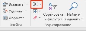
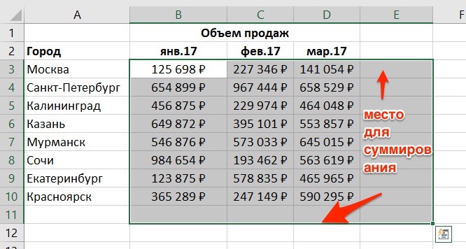
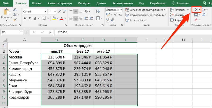
The fastest and by far the easiest way to withdraw an amount in Excel is the AutoSum service. To use it, you need to select the cells that contain the values \u200b\u200bto be added, as well as the empty cell immediately below them. In the "Formulas" tab, click on the "AutoSum" sign, after which the result of addition appears in an empty cell.

Likewise, we drag with the mouse. In the User field, in the row labels area, and the Product field in the column labels area. Thus, the "brief information component" will state the following. Having done the above, the following result will be obtained in the final information component.

How to calculate the amount in a column using the AutoSum button

In the first place, 3 sellers are sold. These are: Alberto, Carlos and Roberto from 00 quetzale. Other uses that can be provided to a dynamic table are as follows. When running a spreadsheet, the user can have results such as: averages, counts, maximums, minimums, variances, among other quantitative field calculations.

The same method is available in reverse order. In an empty cell where you want to display the result of addition, you need to put the cursor and click on the "AutoSum" sign. After clicking in the cell, a formula with a free summation range is formed. Using the cursor, select a range of cells, the values \u200b\u200bof which need to be added, and then press Enter.

One of the great spreadsheet utilities is to generate calculations from qualitative variables or from discrete quantitative variables. These results in the pivot table can be changed and displayed instantly because the fields involved in the field change locations.

Data Format and Import Considerations

You can quickly add a layer to your map by choosing one of the suggested styles. You can choose one of the Quick Map styles, or manually specify your style options, location type, and data source. When you're creating a map, it's easy to get carried away and try to add a lot of data to the map. It's important to keep in mind that tracking too many individual features on a map can be confusing and frustrating for the user and doesn't provide a clear picture of your business data.

Cells for addition can also be defined without cursor selection. The formula for the sum is: "\u003d SUM (B2: B14)", where the first and last cells of the range are given in brackets. By changing the values \u200b\u200bof the cells in the Excel table, you can adjust the summation range.

Sum of values \u200b\u200bfor information

Excel not only allows you to sum values \u200b\u200bfor some specific purpose, but also automatically counts the selected cells. Such information can be useful in cases where the task is not related to the summation of numbers, but consists in the need to look at the value of the sum at an intermediate stage. To do this, without resorting to writing a formula, it is enough to select the necessary cells and in the command line of the program at the very bottom of the right-click on the word "Done". In the context menu that opens opposite the "Amount" column, the value of all cells will be displayed.

How to calculate the amount in a column using the simple addition formula

Data import limits for each level. If your data contains a large number of features, you can add them to the map in subsets, for example, if you have 000 features, create two layers, each containing 1000 points. You can turn off clustering using the Cluster Points button on the map ribbon.

Add quick map layer

The columns in the dataset to be used for the location must be formatted as text values \u200b\u200band not as numeric values. Because of this, unlike true date and time values, time values \u200b\u200bby themselves cannot be used in time animations.

Named tables and ranges.
Use text values.

To add a layer from the suggested styles, follow these steps.

Simple addition formula in Excel

In cases where the values \u200b\u200bfor addition are scattered throughout the table, you can use simple formula addition in Excel-table. The formula has the following structure:

To create a formula in a free cell, where the amount should be displayed, put an equal sign. Excel automatically responds to this action like a formula. Next, using the mouse, you need to select the cell with the first value, after which the plus sign is placed. Further, all other values \u200b\u200bare also entered into the formula through the addition sign. After the chain of values \u200b\u200bis typed, the Enter button is pressed. This method is useful when adding a small amount of numbers.

To select a data source for a map, follow these steps. Several geocoders can be configured and any of them can be set as default. To select a location type, follow these steps. For example, if you want to compare all stores in a franchise based on revenue, select the column that contains information on sales revenue. The carousel shows several ways in which you can compare map entries.

Adding a custom location type

To apply a column style, follow these steps. In the window, click the Style drop-down arrow and select the column to use to style the layer. To assign your entries to specific locations by location only, select. The style settings are updated to display suggested styles based on the specified location type. A confirmation window opens displaying the details for creating the map layer, the selected location type, and the selected style. To turn off confirmation for each new layer, select the Don't show this message again check box. You can re-enable confirmation at any time by changing the setting in the card settings. Click Add Data. The data in your table is added as a layer to the map. If your data contains repeating areas, you have the option to add the data before creating the layer. In the Add Areas section. Select the style you want for your layer and click Add Data. ... Custom limits can include shopping districts, zoning limits, or other specific areas.

SUM formula in Excel

Despite the almost automated process of using addition formulas in Excel, it is sometimes easier to write the formula yourself. In any case, their structure must be known in cases where work is carried out in a document created by another person.

The SUM formula in Excel has the following structure:

To add a location type, follow these steps. If your data contains repeating areas, you have the option to add data from those areas to summarize the information in a way that makes it easier to analyze. For example, if you decide to create a map with the location type of a state, but your data contains sales results from many postal codes in each state, you can summarize the information so that when you click on the map state polygon, the total sales of all postal codes in that state are shown.

SUM (A1; A7; C3)

When typing a formula yourself, it is important to remember that spaces are not allowed in the structure of the formula, and the sequence of characters must be clear.

The sign ";" serves to define a cell, in turn, the ":" sign sets a range of cells.

An important nuance - when calculating the values \u200b\u200bof the entire column, you do not need to set the range, scrolling to the end of the document, which has a border of over 1 million values. It is enough to enter a formula with the following values: \u003d SUM (B: B), where the letters represent the column to be calculated.

Add custom coordinate system

To add data, follow these steps. To add a custom coordinate system, follow these steps. In the window "Add data from table spreadsheets"Select" Coordinates "from the" Place Type "drop-down menu and click" Format Placement ". Use the Longitude and Latitude drop-down menus to select the appropriate data columns and map them to the location fields. Click "Details" to view additional information about the service or objects of the map. The Import Custom Spatial References window opens, displaying information about the selected spatial reference. In the Alias \u200b\u200btext box, enter a unique name for the custom coordinate system. Click Import to import the spatial reference. New system coordinates is displayed at the top of the Other drop-down menu. To define a custom spatial reference as the default when adding data to the map using coordinates, select the Use as default check box. Click OK to return to the Add Data Workflow window.

In the Select Spatial Reference panel, select Others and click Import.
Click Select to select a map or location service.

You can directly correct these errors in the Content panel.

Excel also allows you to display the sum of all cells in the document without exception. To do this, the formula must be entered in a new tab. Suppose that all the cells whose sums need to be calculated are located on Sheet1, in which case the formula should be written on Sheet2. The structure itself is as follows:

SUM (Sheet1! 1: 1048576), where the last value is the numerical value of the most recent cell of Sheet1.

You can create formula cells or functions that automatically perform calculations using data from any group of cells you choose. For example, you can compare the values \u200b\u200bof two cells, calculate the sum or product of multiple cells, etc. the result of the formula or function will be shown in the same cell where you entered the formula or function.

You can also use any of the over 250 predefined math functions included in the pages to create formulas. There are functions for statistical, engineering and financial applications, some of which receive information remotely over the Internet. You will find detailed information about each of these functions in the Function Browser as you type an equal sign in a cell, and in the help information about formulas and functions available on the Internet.

Related Videos

select an area of \u200b\u200bcells;
use the "AutoSum" button;
create a simple addition formula;
using a function.

Calculate the sum by selecting a region of cells

First, you can find out the sum of any cells with values \u200b\u200bsimply by highlighting the cells you need with the left mouse button:

Add, subtract, multiply, or divide values

You can create simple or complex arithmetic formulas to perform calculations based on values \u200b\u200bin your tables.

You can use comparison operators to check if the values \u200b\u200bof two cells are the same, or if one value is greater or less than the other. The result of a comparison operator is expressed as true or false.

By selecting cells with numbers, in the lower right corner Excel will display the sum of the values \u200b\u200bin the range you selected.

In order to select cells that are not in the neighborhood, hold down the CTRL key and select cells with the left mouse button.

How to calculate the amount in a column using the simple addition formula

Perhaps the simplest and most primitive way to sum data in a column is the simple addition formula. To summarize data:

Reference cells in formulas

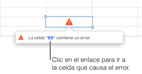
If there is an error in the formula, it will appear in the result cell. Click on it to see the error message. If the message indicates that another cell is causing an error, you can click the cell reference to select the cell with the error.

In formulas, you can include cell references, ranges of cells and columns, or entire rows of data, and even cells in other tables or pages. Pages use the values \u200b\u200bof the reference cells to calculate the result of the formula.

left-click on the cell where you want to get the result of addition;
enter the formula:

In the formula above, specify the numbers of the cells that you want to sum:

How to calculate the amount in a column using the AutoSum button

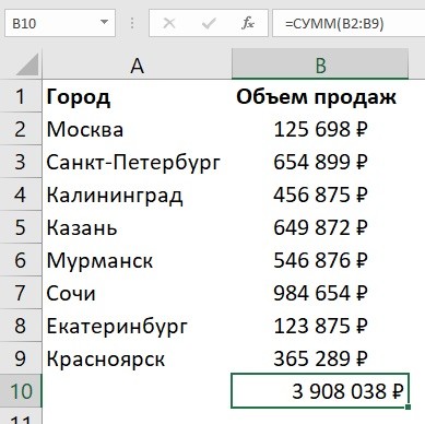
If you want to calculate the sum of the numbers in a column and leave this result in the table, then perhaps the easiest way is to use the AutoSum function. It will automatically determine the range of cells required for the summation and save the result in the table.

Insert functions into cells

The following examples show the use of cell references in formulas. If the reference range spans more than one cell, the start and end cells are separated by a single colon. Note that the table name and cell reference are separated by two colons. When you select a cell in another table for a formula, the table name is automatically included. To refer to a column, you can use the column letter. The following formula calculates the total number of cells in the third column: You can use the row number to refer to a row. The following formula calculates the total number of cells in the first row: To refer to a row or column with a header, you can use the header name.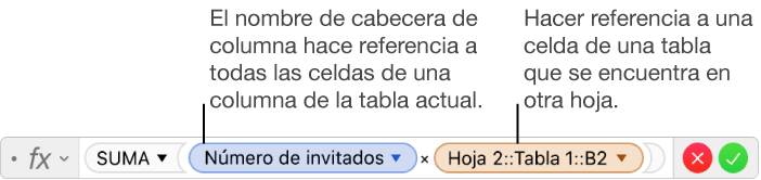

If the referenced cell is from another table, the reference must contain the table name. ... You can use any of the over 250 predefined math functions included in the pages of your document.

To count the numbers in a column using AutoSum, do the following:

click on the first blank cell in the column below the values \u200b\u200byou want to sum:

select the AutoSum icon on the toolbar:

after pressing the button, the system will automatically select the range to add. If the system has chosen the wrong range, you can correct it simply by changing the formula:

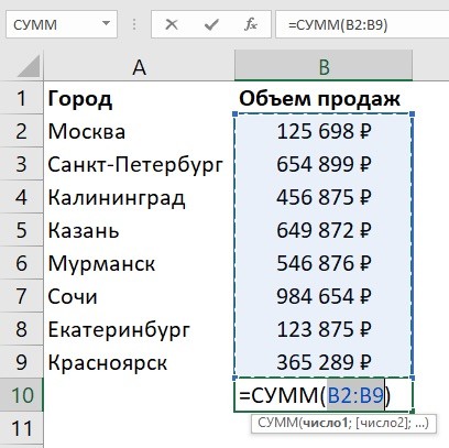
once you are sure that the range of values \u200b\u200bfor the amount is selected correctly, just press the Enter key and the system will calculate the amount in the column:

How to calculate the sum in a column using the SUM function in Excel

You can add the values \u200b\u200bin a column using a function. Most often, the formula is used to create a sum individual cells in a column or when the sum cell should not be located directly below the data column. To calculate the amount using the function, follow these steps:

select a cell with the left mouse button and enter the function ““, specifying the required range of cells:

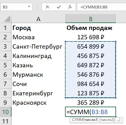
press the “Enter” button and the function will calculate the amount in the specified range.

How to calculate the amount in a column in Excel using a table

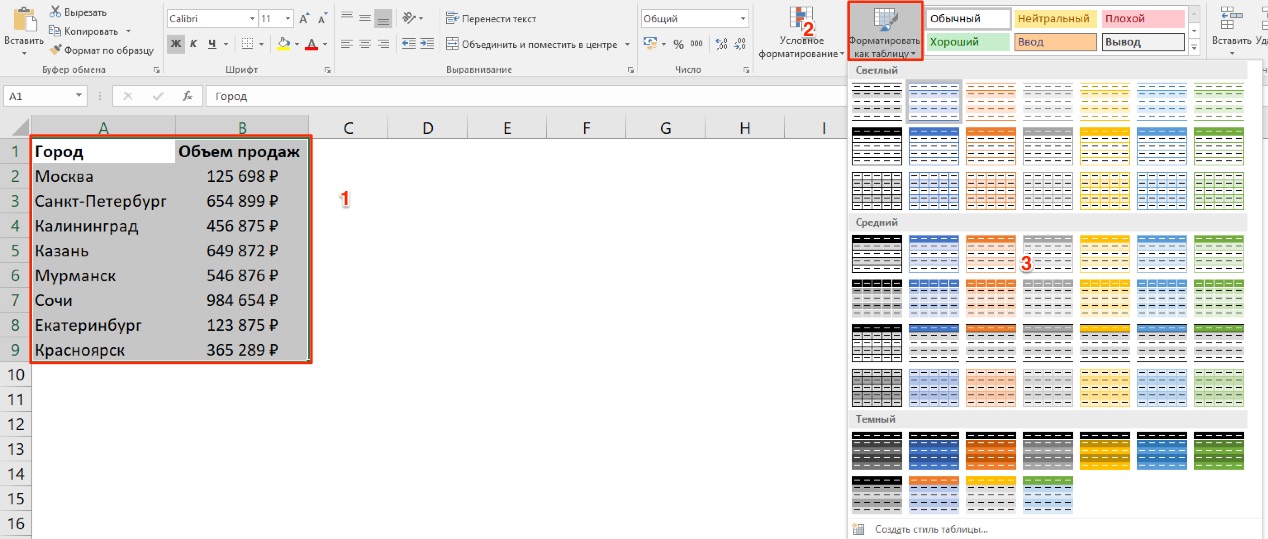
To calculate the amount in a column of data, you can format the data as a table. For this:

select a range of cells with data and convert them to a table using the button on the "Format as Table" toolbar:

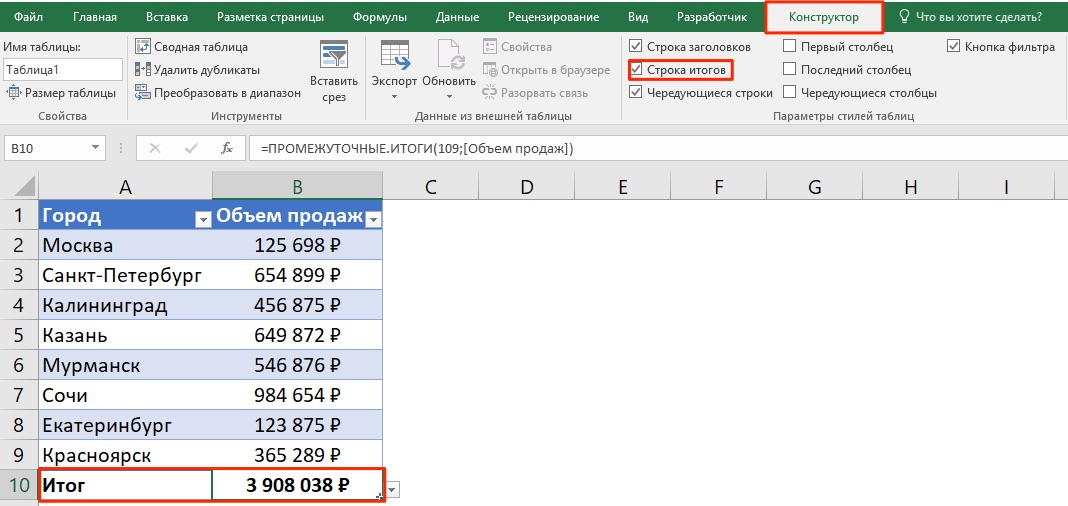
after your data is presented in table format, on the “Design” tab on the toolbar, select the “Total row” item in order to add the sum of the columns under the table: