Sum selected cells in excel. Excel. Count and sum cells that meet conditional formatting criteria
It often happens that you need to sum every second, third, fourth, etc. cell in a spreadsheet. Now, thanks to the next trick, it can be done.
Excel does not provide a standard function that can sum each nth cell or string. However, you can accomplish this task with several different ways... All of these approaches are based on the ROW and MOD functions.
ROW function returns the row number for the given cell reference: ROW (reference), in the Russian version of Excel ROW (reference).
OSTAT function (MOD) returns the remainder of dividing a number by a divisor: MOD (number; divisor), in the Russian version of Excel OSTAT (number; divisor).
Put the ROW function in the MOD function (to pass a numeric argument), divide by 2 (to sum every other cell) and check if the result is not zero. If so, the cell is added up. These functions can be used in a wide variety of ways - some will provide better results than others. For example, an array formula to sum every second cell in the range $ A $ 1: $ A $ 100 might look like this: \u003d SUM (IF (MOD (ROW ($ A $ 1: $ A $ 500); 2) \u003d 0; $ A $ 1: $ A $ 500; 0)), in the Russian version of Excel \u003d SUM (IF (OSTAT (LINE ($ A $ 1: $ A $ 500); 2) \u003d 0; $ A $ 1: $ A $ 500; 0)).
Since this is an array formula, you must enter it by pressing Ctrl + Shift + Enter, Excel will add curly braces so that it looks like this: (\u003d SUM (IF (MOD (ROW ($ A $ 1: $ A $ 500), 2) \u003d 0; $ A $ 1: $ A $ 500; 0))), in the Russian version of Excel: (\u003d SUM (IF (Remaining (ROW ($ A $ 1: $ A $ 500); 2) \u003d 0; $ A $ 1: $ A $ 500; 0))) You need Excel to add curly braces by itself; if you add them yourself, the formula won't work.
Although the goal is achieved, this method negatively affects the design. spreadsheet... This is an unnecessary application of an array formula. To make matters even worse, this long formula includes a recalculable ROW function, which turns a large formula into a recalculable function as well. This means that it will be constantly recalculated, no matter what you do in the workbook. This is a very bad way!
Here is another formula that is slightly the best choice: \u003d SUMPRODUCT ((MOD (ROW ($ A $ 1: $ A $ 500); 2) \u003d 0) * ($ A $ 1: $ A $ 500)), in the Russian version of Excel \u003d SUMPRODUCT ((REST (ROW ($ A $ 1 : $ A $ 500); 2) \u003d 0) * ($ A $ 1: $ A $ 500)).
Remember, however, that this formula will return the #VALUE! (#VALUE!) If any cells in the range contain text instead of numbers. This formula, while not actually an array formula, also slows down excel workif you use it too many times, or if it refers to a large range each time.
Fortunately there is the best way, which is not only more efficient, but also much more flexible. It requires the use of the DSUM function. In this example, we used the range A1: A500 as the range over which every nth cell needs to be added.
Enter the word Criteria in cell E1. Enter the following formula in cell E2: \u003d MOD (ROW (A2) - $ C $ 2-1; $ C $ 2) \u003d 0, in the Russian version of Excel \u003d OSTAT (ROW (A2) - $ C $ 2-1; $ C $ 2) \u003d 0. Select cell C2 and select the Data → Validation command.
In the Allow field, select List, and in the Source field, enter 1, 2, 3, 4, 5, 6, 7, 8, 9, 10. Make sure the List box is checked acceptable values (In-Cell), and click the OK button. In cell C1, enter the text SUM every…. In any cell other than row 1, enter the following formula: \u003d DSUM ($ A: $ A; 1; $ E $ 1: $ E $ 2), in the Russian version of Excel \u003d BDSUMM ($ A: $ A; 1; $ E $ 1 : $ E $ 2).
In the cell directly above the cell where you entered the DSUM function, enter the text \u003d "Summing Every" & $ C $ 2 & CHOOSE ($ C $ 2; "st"; "nd"; "rd"; "th"; " th ";" th ";" th ";" th ";" th ";" th ") &" Cell ". Now all that remains is to select the desired number in cell C2, and the DSUM function will do the rest.
Using the function BDSUM (DSUM), you can sum cells at the interval you specify. The DSUM function is much more efficient than an array formula or the SUMPRODUCT function. Although it takes a little longer to set up, this is the case when it's hard to learn, easy to fight.
Earlier I described how to find a. Unfortunately, this function does not work if cells are colored with conditional formatting... I promised to "refine" the function. But in the two years that have passed since the publication of that note, I have not been able to write digestible code either on my own or with the help of information from the Internet ... ( Update March 29, 2017 After another five years, I still managed to write the code; see the final part of the note). And just recently I came across an idea contained in the book by D. Hawley, R. Hawley "Excel 2007. Tricks", which allows you to do without code.
Let there be a list of numbers from 1 to 100, located in the range A1: A100 (Fig. 1; see also the "SUMIF" sheet of the Excel file). The range has been conditionally formatted to mark cells that contain numbers greater than 10 and less than or equal to 20.
Figure: 1. Range of numbers; conditional formatting highlighted cells containing values \u200b\u200bfrom 10 to 20
Download note in format, examples in format
Now you need to add the values \u200b\u200bin the cells that meet the criteria just set. It doesn't matter what kind of formatting is applied to these cells, but you need to know the criteria by which the cells are highlighted.
To add up a range of cells that match one criterion, you can use the SUMIF function (Fig. 2).
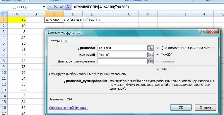
Figure: 2. Summation of cells that meet one condition
If you have some conditions, you can use the SUMIFS function (Fig. 3).

Figure: 3. Summing cells that meet several conditions
You can use the COUNTIF function to count the number of cells that match one criterion.
You can use the COUNTIF function to count the number of cells that meet multiple criteria.
Excel provides another function that allows you to specify multiple conditions. This function is included in the set of functions of bases excel data and is called BDSUMM. To check it, use the same set of numbers in the range A2: A100 (Fig. 4; see also the "BDSUMM" sheet of the Excel file).
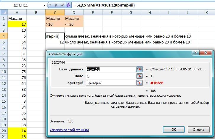
Figure: 4. Using database functions
Select cells C1: D2 and name this range Criterion by typing it in the name box to the left of the formula bar. Now select cell C1 and enter \u003d $ A $ 1, which is a reference to the first cell on the sheet containing the name of the database. Enter \u003d $ A $ 1 in cell D1 and you will get two copies of the column heading A. These copies will be used as headers for the conditions BDSUMM (C1: D2), which you named Criterion. In cell C2, enter\u003e 10. In cell D2, enter<=20. В ячейке, где должен быть результат, введите следующую формулу:
BDSUMM ($ A $ 1: $ A $ 101.1, Criterion)
You can use the COUNT function to count the number of cells that meet multiple criteria.
Reading the book by John Walkenbach, I learned that starting with Excel 2010, VBA has a new DisplayFormat property (see, for example, Range.DisplayFormat Property). That is, VBA can read the format displayed on the screen. It does not matter how it was received by direct user settings, or using conditional formatting. Unfortunately, MS has made it so that the DisplayFormat property only works in procedures called from VBA, and UDFs based on this property throw a #VALUE! However, you can get the sum of values \u200b\u200bin a range by cells of a certain color using a procedure (a macro, but not a function). Open (contains VBA code). Go through the menu View -> Macros -> Macros; in the window Macro, highlight the line SumColorUsl, and press Execute... Run the macro, select the summation range and criterion. The answer will appear in the window.
Procedure code
Sub SumColorConv () Application.Volatile True Dim SumColor As Double Dim i As Range Dim UserRange As Range Dim CriterionRange As Range SumColor \u003d 0 "Range query Set UserRange \u003d Application.InputBox (_ Prompt: \u003d" Select summation range ", _ Title: \u003d "Range Selection", _ Default: \u003d ActiveCell.Address, _ Type: \u003d 8) "Criterion Request Set CriterionRange \u003d Application.InputBox (_ Prompt: \u003d" Select summation criterion", _ Title: \u003d" Criterion selection ", _ Default: \u003d ActiveCell.Address, _ Type: \u003d 8)" Summing the "correct" cells For Each i In UserRange If i.DisplayFormat.Interior.Color \u003d _ CriterionRange.DisplayFormat. Interior.Color Then SumColor \u003d SumColor + i End If Next MsgBox SumColor End Sub
Sub SumColorUl () Application. Volatile True Dim SumColor As Double Dim i As Range Dim UserRange As Range Dim CriterionRange As Range SumColor \u003d 0 "Range query Set UserRange \u003d Application.InputBox (_ Prompt: \u003d "Select summation range", _ Title: \u003d "Range selection", _ Default: \u003d ActiveCell.Address, _ Type: \u003d 8) "Proscriptor Set CriterionRange \u003d Application. InputBox (_ Prompt: \u003d "Select a summation criterion", _ Title: \u003d "Criterion selection", _ Default: \u003d ActiveCell. Address, _ |
Suppose you have a sales report like this:
From it you need to find out how much pencils sold by sales representative Ivanov in january.
PROBLEM: How to summarize data by several criteria ??
DECISION: Method 1:
BDSUMM (A1: G16; F1; I1: K2)
In the English version:
DSUM (A1: G16, F1, I1: K2)
HOW IT WORKS:
From the database we specified A1: G16 function BDSUMM retrieves and summarizes column data amount (argument " Field" = F1) according to the given in cells I1: K2 (Seller \u003d Ivanov; Products \u003d Pencils; Month \u003d January) criteria.
CONS: The list of criteria should be on the sheet.
NOTES: The number of summation criteria is limited by the RAM.
APPLICATION AREA: Any version of Excel
Method 2:
SUMPRODUCT ((B2: B16 \u003d I2) * (D2: D16 \u003d J2) * (A2: A16 \u003d K2) * F2: F16)
In the English version:
SUMPRODUCT ((B2: B16 \u003d I2) * (D2: D16 \u003d J2) * (A2: A16 \u003d K2) * F2: F16)
HOW IT WORKS:
The SUMPRODUCT function forms arrays of TRUE and FALSE values, according to the selected criteria, in Excel memory.

If the calculations were performed in the cells of the sheet (for clarity, I will demonstrate the whole work of the formula as if the calculations are taking place on the sheet, and not in memory), then the arrays would look like this:

It is obvious that if, for example, D2 \u003d Pencils, then the value will be TRUE, and if D3 \u003d Folders, then FALSE (since the criterion for selecting a product in our example is the value The pencils).
Knowing that TRUE is always equal to 1, and FALSE is always equal to 0, we continue to work with arrays as with numbers 0 and 1.
Multiplying the obtained values \u200b\u200bof the arrays with each other sequentially, we get ONE array of zeros and ones. Where all three selection criteria were met, ( IVANOV, PENCILS, JANUARY) i.e. all conditions took on the values \u200b\u200bTRUE, we get 1 (1 * 1 * 1 \u003d 1), but if at least one condition is not met, we get 0 (1 * 1 * 0 \u003d 0; 1 * 0 * 1 \u003d 0; 0 * 1 * 1 \u003d 0).
Now it remains only to multiply the resulting array by an array containing data that we need to sum up as a result (range F2: F16) and, in fact, sum up what is not multiplied by 0.
Now compare the arrays obtained using the formula and during the step-by-step calculation on the sheet (highlighted in red).
I think everything is clear :)
MINUSES: SUMPRODUCT - "heavy" array formula. When calculating on large data ranges, the recalculation time noticeably increases.
NOTES
APPLICATION AREA: Any version of Excel
Method 3: Array Formula
SUM (IF ((B2: B16 \u003d I2) * (D2: D16 \u003d J2) * (A2: A16 \u003d K2); F2: F16))
In the English version:
SUM (IF ((B2: B16 \u003d I2) * (D2: D16 \u003d J2) * (A2: A16 \u003d K2), F2: F16))
HOW IT WORKS: In the same way as Method # 2. There are only two differences - this formula is entered by pressing Ctrl + Shift + Enterrather than just pressing Enter and the array 0-th and 1-q is not multiplied by the summation range, but is selected using the IF function.
MINUSES: Array formulas when computing large data ranges noticeably increase the recalculation time.
NOTES: The number of processed arrays is limited to 255.
APPLICATION AREA: Any version of Excel
Method 4:
SUMIF (F2: F16; B2: B16; I2; D2: D16; J2; A2: A16; K2)