How to compare two columns in Excel - Excel data comparison methods
This is a chapter from the book: Michael Girwin. Ctrl + Shift + Enter. Mastering array formulas in Excel.
Samples based on one or more conditions.Row excel functions use comparison operators. For example, SUMIF, SUMIFS, COUNTIF, COUNTIFS, AVERAGEIF, and AVERAGEIFS. These functions make selections based on one or more conditions (criteria). The problem is that these functions can only add, count, and average. What if you want to impose conditions on your search, such as maximum value or standard deviation? In these cases, since there is no built-in function, you must invent an array formula. This is often due to the use of the array comparison operator. The first example in this chapter shows how to calculate the minimum value under one condition.
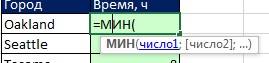
Let's use the IF function to select array elements that meet a condition. In fig. 4.1 in the left table there is a column with city names and a column with time. It is required to find the minimum time for each city and place this value in the corresponding cell of the right table. The condition for the selection is the name of the city. If you use the MIN function, you can find the minimum value for column B. But how do you select only those numbers that are specific to Oakland? And how do you copy the formulas down the column? Since Excel does not have a built-in MINESLI function, you need to write an original formula that combines the IF and MIN functions.
Figure: 4.1. Purpose of the formula: choose the minimum time for each city
Download a note in format or format
As shown in fig. 4.2, you should start entering the formula in cell E3 with the MIN function. But you cannot put in an argument number1 all values \u200b\u200bin column B !? You want to select only those values \u200b\u200bthat are specific to Auckland.
As shown in fig. 4.3, in the next step, enter the IF function as an argument number1 for MIN. You put IF inside MIN.
By placing the cursor where the argument is entered log_expression function IF (Fig. 4.4), you select a range with city names A3: A8, and then press F4 to make cell references absolute (see, for example, for more details). Then you type the comparison operator, the equal sign. Finally, you will select the cell to the left of the formula - D3, keeping the reference to it relative. The formulated condition will allow you to select only Aucklands when viewing the range A3: A8.

Figure: 4.4. Create array operator on argument log_expression functions IF
So you've created an array operator using the comparison operator. At any point in the processing of an array, the array operator is a comparison operator, so its result will be an array of TRUE and FALSE values. To verify this, select the array (to do this, click in the tooltip on the argument log_expression) and press F9 (fig. 4.5). You usually use one argument log_expression, returning either TRUE or FALSE; here, the resulting array will return multiple TRUE and FALSE values, so the MIN function will only select the minimum number for cities that match the TRUE value.
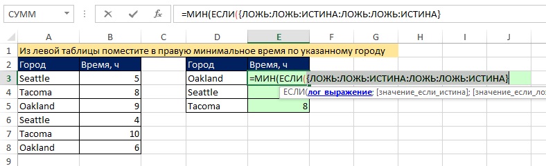
Figure: 4.5. To see an array of TRUE and FALSE values, click on the argument in the tooltip log_expression and press F9
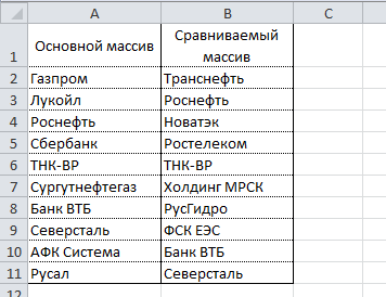
We have two tables of orders copied into one worksheet. It is necessary to compare the data of two tables in Excel and check which positions are in the first table, but not in the second. There is no point in manually comparing the value of each cell.
Compare two columns for matches in Excel
How to make comparison of values \u200b\u200bin Excel of two columns? To solve this problem, we recommend using conditional formattingto quickly highlight items that are in only one column. Worksheet with tables:
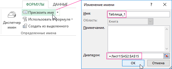
The first step is to assign names to both tables. This makes it easier to understand which cell ranges are being compared:
- Select the FORMULAS tool - Defined Names - Assign Name.
- In the window that appears, in the "Name:" field, enter the value - Table_1.
- Left-click on the "Range:" entry field and select the range: A2: A15. And click OK.
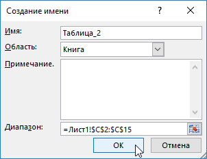
For the second list, do the same, but assign a name - Table_2. And indicate the range C2: C15 - respectively.
Useful advice! Range names can be assigned more quickly by using the name field. It is located to the left of the formula bar. Just select the ranges of cells, and in the name field, type the appropriate name for the range and press Enter.

Now let's use conditional formatting to compare two lists in Excel. We need to get the following result:
Positions that are in Table_1, but not in Table_2 will be displayed in green. At the same time, the positions located in Table_2, but absent in Table_1, will be highlighted in blue.


Principle of comparing data of two columns in Excel
We used the COUNTIF function to define the conditions for formatting the column cells. In this example, this function checks how many times the value of the second argument (for example, A2) occurs in the list of the first argument (for example, Table_2). If the number of times \u003d 0 then the formula returns TRUE. In this case, the cell is assigned the custom format specified in the conditional formatting options. The reference in the second argument is relative, which means that all cells of the selected range will be checked in turn (for example, A2: A15). The second formula works in a similar way. The same principle can be applied to various similar tasks. For example, to compare two prices in Excel, even
When working in Excel, a fairly common task is to compare different kinds of lists of values. Standard Excel tools such as conditional formatting and functions can be used to compare ranges of values \u200b\u200bin general and columns of values \u200b\u200bin particular. In addition, you can solve such tasks using VBA macros and add-ins for Excel based on them.
The need to compare ranges in general and columns in particular arises when updating various reports, lists and databases generated in Excel and requiring changes over time.IN internet networks quite a lot of examples have been described that use various functions (formulas) and conditional formatting to compare values \u200b\u200bin columns. For those for whom such methods are not suitable for any reason, you can use another tool that allows you to compare both columns and any ranges of values \u200b\u200bconsisting of any number of rows and columns. With the help of the add-in for Excel, you can compare any two ranges, or, more precisely, compare each element of one range with each element of the other and find both the matches and differences between them of your choice.
Excel comparison add-in for values \u200b\u200bin two ranges
The add-on, which will be discussed below, is designed to compare values \u200b\u200bin two ranges, consisting of any number of rows and columns. This add-in uses the procedure of comparing each element of one range with each element of another range, determines which elements of these ranges are the same and which are different, and fills the cells with a user-specified color.
As you can see from the dialog box, everything is quite simple, the user selects two ranges to be compared, determines what to look for, different values \u200b\u200bor the same, selects a color and launches the program. The end result of using the add-in is filled cells with a specific color, indicating differences or overlaps in the values \u200b\u200bof the selected ranges.
There is one nuance when comparing values \u200b\u200bin Excel. Numbers can be formatted as text, which is not always visually identifiable (). That is, a number in Excel can be either a numerical value or a text value, and these two values \u200b\u200bare not equal to each other. Very often this phenomenon causes various kinds of errors. In order to exclude such errors, the "Compare numbers as text" option is used, which is enabled by default. Using this option allows you to compare not numeric values, but converted text values.
The add-on allows:
1. With one mouse click, open the macro dialog box directly from the Excel toolbar;
2. find elements of range # 1 that are not in range # 2;
3. find elements of range # 2 that are not in range # 1;
4. find elements of range # 1 that are in range # 2;
5. find elements of range # 2 that are in range # 1;
6. choose one of nine fill colors for the cells with the desired values;
7. quickly select ranges using the "Limit ranges" option, while you can select entire rows and columns, reducing the selected range to the used one is done automatically;
8. instead of comparing numeric values, use comparison of text values \u200b\u200busing the "Compare numbers as text" option;
9. compare values \u200b\u200bin the cells of the range without taking into account extra spaces;
10.Compare values \u200b\u200bin cells of a range in a case-insensitive manner.
How to compare two columns using a macro (add-in) for Excel?
Column comparison is a special case of comparing arbitrary ranges. In ranges # 1 and # 2, select two columns, and you can select exactly the columns, and not drag the selection frame over the ranges with cells with the mouse (for convenience, the "Limit Ranges" option is enabled by default, selection using the range), select the required action to search for either differences or matches, select the fill color of the cells and run the program. Below you can see the result of searching for matching values \u200b\u200bin two columns.
The ability to compare two datasets in Excel is often useful for people processing large amounts of data and working with huge tables. For example, comparison can be used in, the correctness of entering data or entering data into a table on time. The article below describes several techniques for comparing two columns with data in Excel.
Using the IF conditional operator
The method of using the conditional operator IF differs in that only the part necessary for comparison is used to compare two columns, and not the entire array. Below are the steps to implement this method:
Place both columns for comparison in columns A and B of the worksheet.
In cell C2, enter the following formula \u003d IF (ISERROR (SEARCH (A2; $ B $ 2: $ B $ 11; 0)); ""; A2) and extend it to cell C11. This formula sequentially searches for each item from column A in column B and returns the item's value if found in column B.

Using the VLOOKUP substitution formula
The principle of the formula is similar to the previous method, the difference lies in, instead of SEARCH. A distinctive feature of this method is also the ability to compare two horizontal arrays using the HLP formula.
To compare two columns with the data in columns A and B (similar to the previous method), enter the following formula \u003d VLOOKUP (A2; $ B $ 2: $ B $ 11; 1; 0) into cell C2 and drag it to cell C11.

This formula looks at each element from the main array in the compared array and returns its value if it was found in column B. Otherwise, Excel will return a # N / A error.
Using VBA Macro
Using macros to compare two columns can unify the process and reduce data preparation time. The decision about which comparison result should be displayed depends entirely on your imagination and skills in using macros. Below is the technique published on the official Microsoft website.
1 | Sub Find_Matches () |
In this code, the CompareRange variable is assigned a range with the compared array. It then runs a loop that loops through each item in the selected range and compares it to each item in the range being compared. If elements with the same values \u200b\u200bwere found, the macro enters the value of the element in column C.
To use the macro, return to the worksheet, select the main range (in our case, these are cells A1: A11), press Alt + F8. In the dialog that appears, select the macro Find_Matchesand click the execute button.

After executing the macro, the result should be as follows:
![]()
Using the Inquire add-in
Outcome
So, we looked at several ways to compare data in Excel that will help you solve some analytical problems and make it easier to find duplicate (or unique) values.
When comparing several comparable items in Excel spreadsheets, the data is often organized in columns so that it is convenient to compare the characteristics of these objects line by line. For example, car models, telephones, experimental and control groups, a number of retail chain stores, etc. With a large number of lines, visual analysis cannot be reliable. Functions VLOOKUP, INDEX, SEARCH (VLOOKUP, INDEX, MATCH) are convenient for comparing data on cells and do not give an overall picture. How do you find out how similar the columns are in general? Are the columns identical?
The Map Columns add-in lets you map columns and see the big picture:
- Compare two or more columns with each other
- Compare Columns with Reference Values
- Calculate the exact match percentage
- Present the result in a visual pivot table
Video language: English. Subtitles: Russian, English. (Attention: video may not reflect latest updates... Use the instructions below.)
Add "Match Columns" to Excel 2016, 2013, 2010, 2007
Suitable for: Microsoft Excel 2016 - 2007, desktop Office 365 (32-bit and 64-bit).
How to work with the add-in:
How to compare two or more columns with each other and calculate the percentage of match
Consider a product development example. Suppose you need to compare several finished prototypes with each other and find out how similar, different, and possibly even identical they are.
- Click the Map Columns button in the XLTools toolbar\u003e Select Map Columns to Each other.
- Click OK\u003e
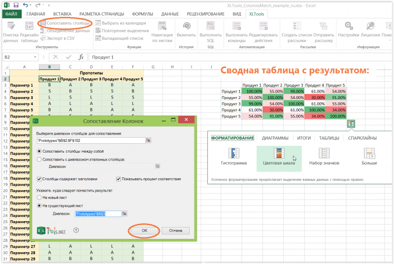
Advice:
Please select summary table result\u003e Click on the Express Analysis icon\u003e Apply "Color Scale".
Reading the result: prototypes Type 1 and Type 3 are almost identical, the 99% match rate means that 99% of their parameters in the lines are the same. Type 2 and Type 4 are the least similar - their parameters coincide only by 30%.
How to compare columns with reference values \u200b\u200band calculate the degree of match
Consider a product development example. Suppose you need to compare several finished prototypes with a certain target standard, and also calculate the degree to which the prototypes meet these standards.
- Select columns to compare.
For example, columns with prototype data. - Click the Map Columns button in the XLTools toolbar.
- Select Map to Reference Column Range\u003e Select Reference Columns.
For example, columns with standards. - Check "Columns contain titles" if so.
- Check "Show match percentage" to display the match percentage as a percentage.
Otherwise, the result is displayed as 1 (full match) or 0 (no match). - Indicate where the result should be placed: on a new sheet or on an existing sheet.
- Click OK\u003e Finish, the result is shown in the pivot table.
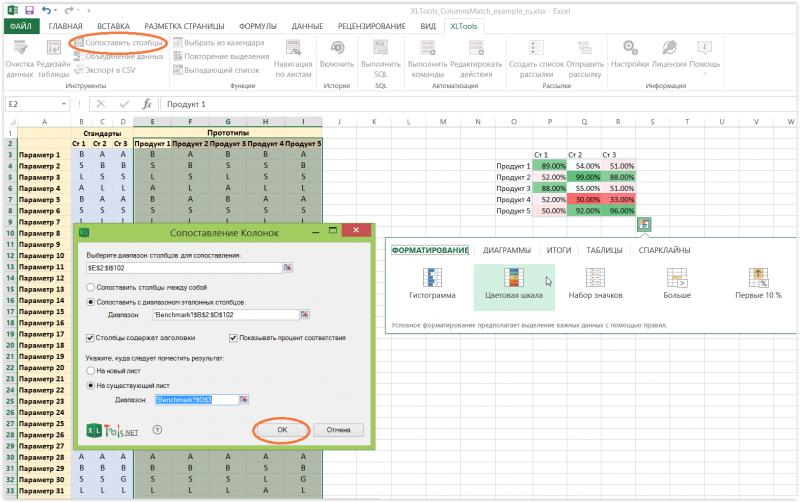
Advice: To make it easier to interpret the result, apply conditional formatting to it:
Select the pivot table of the result\u003e Click on the Quick Analysis icon\u003e Apply "Color Scale".
Reading the result: prototype Type 2 is 99% compliant with Standard 2, i.e. 99% of their parameters in strings are the same. Product 5 is closest to Standard 3 - 96% of their parameters are identical. At the same time, Product 4 is far from meeting any of the three standards. Now we can conclude how much each of the prototypes deviates from the target reference values.
What tasks will the Match Columns add-in help with?
The add-in scans the cells line by line and calculates the percentage of identical values \u200b\u200bin the columns. XLTools Match Columns is not suitable for normal comparison of values \u200b\u200bin cells - it is not designed to find duplicates or unique values.
The Map Columns add-in has a different purpose. Her the main task - find out how, in general, the datasets (columns) are similar or different. The add-on helps with the analysis of a large amount of data when you need to look at a broader macro level, for example. answer the following questions:
- How similar are the performance of the experimental groups
- How similar are the results of the experimental and control groups
- How similar / different are several products of the same category
- How close are the KPIs of employees to the planned indicators?
- How similar are the indicators of several retail stores, etc.