Excel tables ready

Tables are an important feature of Excel, but many people don't use them too much. This note describes how to work with the table, lists its advantages and disadvantages. A table is a rectangular range of cells containing structured data. Each row in the table corresponds to one object. For example, a line might contain information about a customer, bank transaction, employee, or product. Each column contains a specific piece of information. So, if in each line we have information about an individual employee, then the columns may contain details of information about him - surname, number, date of hiring, salary, department. At the top of the table is a header row that describes the data contained in each column.

Figure: 1. Data range: (a) in the usual representation; (b) in the form of a table

Download a note in format or, examples in format

You have probably created ranges that match this description (Fig. 1a). The fun begins when you want Excel to convert a range of data into a “real” table. To do this, select any cell in the range and run the command Insert –> Tables –> Table, or press Ctrl + T (English) (Fig. 1b).

If you have explicitly converted a range to a table, then Excel will intelligently react to the actions you take in that range. For example, if you create a chart from a table, it will automatically expand as new rows are added to the table. If you create a pivot table from such a table, then after updating the pivot table will be automatically replenished with all the new data that you have added.

Comparing a Range to a Table

Difference between normal range of cells and range converted to table:

By activating any cell in the table, you get access to a new contextual tab Working with tableslocated on the tape.
You can quickly apply formatting (fill color and font color) by choosing an option from the gallery. This formatting is optional.
Each table header has a filter button, by clicking which you can easily sort rows or filter data, hiding those that do not meet the specified criteria.
You can create a "slice" to a table, with which a beginner can quickly apply filters to data. Slices work the same way as with summary tables (see details).
If you scroll the sheet so that the heading row disappears from view, the headings appear in place of the column letters. In other words, you don't have to hard-code the top row to view the column names.
If you create a chart from table data, the chart will automatically expand when new rows are added to the table.
Calculated columns are supported in tables. A formula entered once in a cell will automatically apply to all cells in that column.
Tables support structured formula references that are outside the table. Formulas can use other table names and column headings instead of cell references.
If you hover over the lower-right corner of the lower-right cell in the table, you can click and drag the border to increase the size of the table, either horizontally (adding additional columns) or vertically (additional rows).
It is easier to highlight rows and columns in a table than in a normal range.

Unfortunately, there are limitations when working with tables. If the workbook contains at least one table, some excel functions unavailable:

Does not work Representation (View –> Modesviewingbooks –> Representation).
The book cannot be provided For sharing (Peer review –> Changes –> Accesstobook).
Cannot automatically insert subtotals ( Data –> Structure –> Intermediatethe outcome).
Cannot use array formulas in a table.

Summing up the table

Consider a table with sales statistics (Fig. 2). First, data was entered, and then the range was converted to a table using the command Insert –> Tables –> Table... Without taking any action, the table was named. In our case Table3.

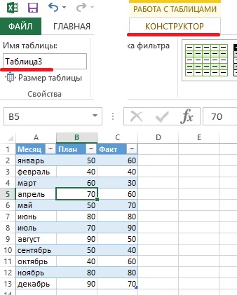
Figure: 2. Simple table with three columns

Activate any cell in the table.
Run the command Working with tables –> Constructor –> Optionsstylestables–> Lineoutcomes and check the box Totals line.
Activate a cell in the totals row and select a summarizing formula from the drop-down list (Figure 3).

Figure: 3. From the drop-down list, you can select a formula to summarize

For example, to calculate the sum of the measures from the column Fact, select option Amount from the drop-down list in cell D14. Excel creates the formula: \u003d INTERMEDIATE.TOTALS (109; [Fact]). Argument 109 corresponds to the SUM function. The second argument to the INTERMEDIATE.TOTALs function is the column name, indicated in square brackets. Using the column name in square brackets allows you to create structured references in the table. The functions of totals in different columns of a table can be different. Option Other functions allows you to construct a fairly complex formula.

You can enable or disable the display of the total row using the command Working with tables –> Constructor –> Optionsstylestables –> Totals line.

Using formulas in a table

In many cases, you need to use formulas in your spreadsheet. For example, in a spreadsheet (see Figure 3), you might want a column that records the difference between actual and planned sales for each month. For this:

Activate cell D1 and enter the word as the column heading Difference - Excel will automatically expand the table.
Go to cell D2, enter the equal sign (start writing the formula), click on cell C2, on the minus sign, and on cell B2.
Press Enter to complete the formula. Formula \u003d [@Fact] - [@ Plan] is entered in all cells of the column.

Instead of the traditional input of a formula using the mouse (as described in section 2), a very convenient way of entering formulas using the keyboard is available in the table. Start with an equal sign, then press the key<– (влево) чтобы указать на соответствующее значение в столбце Fact, enter a minus sign, then double-tap<–, чтобы указать на соответствующее значение в столбце Plan, press Enter to complete the formula.

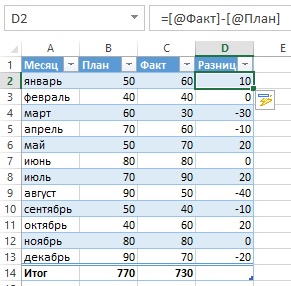
Figure: 4. In the column Difference contains the formula

Each time you enter it into a table, the formula is applied to the entire column. If the formula needs to be changed, edit any formula in the column and the changes will apply to all other formulas in that column.

Auto-propagating a formula to all cells in a table column is one of the auto-correction features in Excel. To disable this feature, click on the icon that appears when entering a formula and select the option Don't automatically create calculated columns(fig. 5).

Figure: 5. The option to automatically create formulas in all cells of the column can be disabled

In the above steps, we used the column headings when creating the formula. For example, you can enter D2 directly in the formula bar into cell D2: \u003d C2-D2. If you enter cell references, Excel will still automatically copy the formula to other cells in the column.

How to reference data in a table

Formulas outside a table can refer to data in that table by its name and column heading. You do not need to create the names of these elements yourself. As usual, click on the desired cells, writing down the formula. The use of table links has a significant advantage: when the table is resized (by deleting or adding rows), the names in it are automatically adjusted. For example, to calculate the sum of all the data in the table in Fig. 2, it is enough to write the following formula: \u003d SUM (Table3). This formula always returns the sum of all data, even if rows or columns of the table are added or removed. If you change the name of Table3, Excel will automatically correct formulas that refer to it.

Typically, you need to refer to a specific column in the table. The following formula returns the sum of the data from the Fact column (but ignores the totals row): \u003d SUM (Table3 [Fact]). Please note that the column name is enclosed in square brackets. Again, the formula adjusts automatically if you change the text in the column header. What's more, Excel provides a hint when you create a formula that refers to data in a table (Figure 6). Formula auto-completion helps you write a formula by displaying a list of items in the table. As soon as you enter an open square bracket, Excel will suggest available arguments.

Figure: 6. Ability to automatically complete formulas when creating formulas that refer to information in a table

Automatic numbering of table rows

In some situations, you might want the rows in the table to be numbered sequentially. You can take advantage of the ability to create calculated columns and write a formula that automatically numbers the columns (Figure 7).

Figure: 7. The numbers in column B are generated using a formula; to enlarge the image, right-click on it and select Open picture in a new tab

As usual, you can enter a calculated column formula in any cell in the column \u003d ROW () - ROW (Table4) +1. When you enter a formula, it automatically propagates to all other cells in the column room... If the LINE function is used without an argument, it returns the string containing the formula. If this function has an argument consisting of a multi-line range, it returns the first row of the range.

The table name contains the first row following the header area. So, in this example, the first row in table Table4 is row 3. The numbers in the table are consecutive row numbers, not data row numbers. For example, when sorting a table, the numbers will remain sequential and will no longer be associated with the same data rows as at the start.

If you filter a table, rows that do not meet the specified criteria will be hidden. In this case, some rows of the table will become invisible (Fig. 8).

Figure: 8. After filtering, the table row numbers are no longer sequential

If you want the table row numbers to remain consistent after filtering, you need a different formula. In cell B3, enter: \u003d INTERMEDIATE.TOTALS (3, C $ 3: C5). The first argument, 3, corresponds to the COUNT function. The INTERMEDIATE.TOTALS function ignores hidden lines, so only visible lines are counted. The formula already refers to column C. This is necessary to avoid the "circular reference" error (Figure 9).

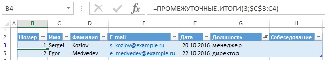
Figure: 9. After filtering, the table row numbers remained sequential

Adapted from the book by John Walkenbach. Excel 2013.. - SPb .: Peter, 2014. - S. 211–220.

Tables in Excel are a series of rows and columns of related data that you manage independently of each other.

With the help of tables you can create reports, make calculations, build graphs and charts, sort and filter information.

If your job is data processing, Excel spreadsheet skills can save you a lot of time and improve efficiency.

How to make a table in Excel. Step-by-step instruction

Data should be organized in rows and columns, with each row containing information about one record, such as an order;
The first row of the table should contain short, unique headings;
Each column must contain one data type, such as numbers, currency, or text;
Each line should contain data for one record, for example, an order. If applicable, provide a unique identifier for each line, such as order number;
The table should not have empty rows and absolutely empty columns.

1. Select an area of \u200b\u200bcells to create a table

Select the area of \u200b\u200bcells where you want to create a table. The cells can be either empty or with information.

2. Click the "Table" button on the Quick Access Toolbar

On the Insert tab, click the Table button.

3. Select a range of cells

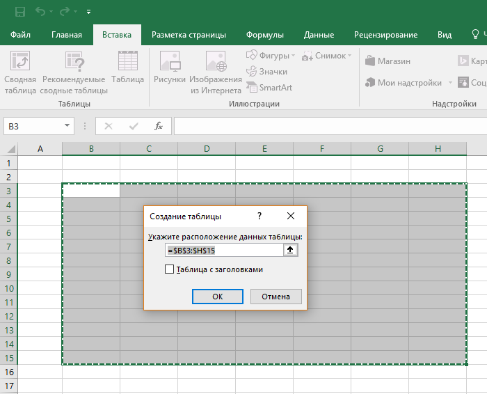
In the popup, you can adjust the location of the data, as well as customize the display of titles. When you're done, click OK.

4. The table is ready. Fill with data!

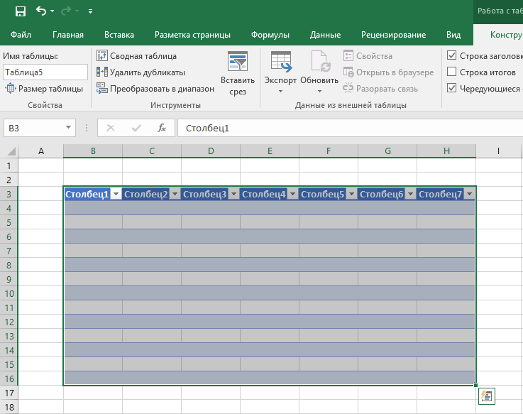
Congratulations, your spreadsheet is now complete! You will learn about the basic features of working with smart tables below.

Preset styles are available for customizing the table format in Excel. All of them are located on the "Design" tab in the "Table Styles" section:

If 7 styles are not enough for you to choose, then by clicking on the button in the lower right corner of the table styles, all available styles will open. In addition to the styles preset by the system, you can customize your format.

In addition to the color scheme, in the "Constructor" menu of tables you can customize:

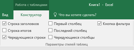
Display header row - enables and disables headers in the table;
Total row - enables and disables the row with the sum of the values \u200b\u200bin the columns;
Alternating lines - highlights alternating lines with color;
First Column - Bolds the text in the first data column;
Last Column - Bolds the text in the last column;
Alternating Columns - highlights alternating columns with color;
Filter Button - Adds and removes filter buttons in the column headers.

How to add a row or column to an Excel table

Even inside an already created table, you can add rows or columns. To do this, right-click on any cell to open a pop-up window:

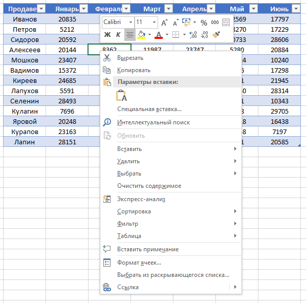
Select “Insert” and left-click on “Table columns on the left” if you want to add a column, or “Table rows above” if you want to insert a row.

If you want to delete a row or column in a table, then go down the list in the pop-up window to the “Delete” item and select “Table Columns” if you want to delete a column or “Table Rows” if you want to delete a row.

How to sort a table in Excel

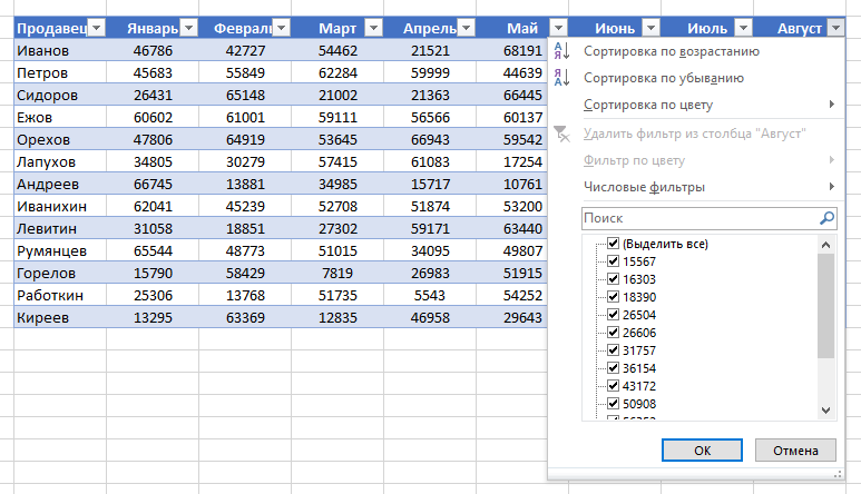
To sort the information in the table, click the “arrow” to the right of the column heading, after which a pop-up window will appear:

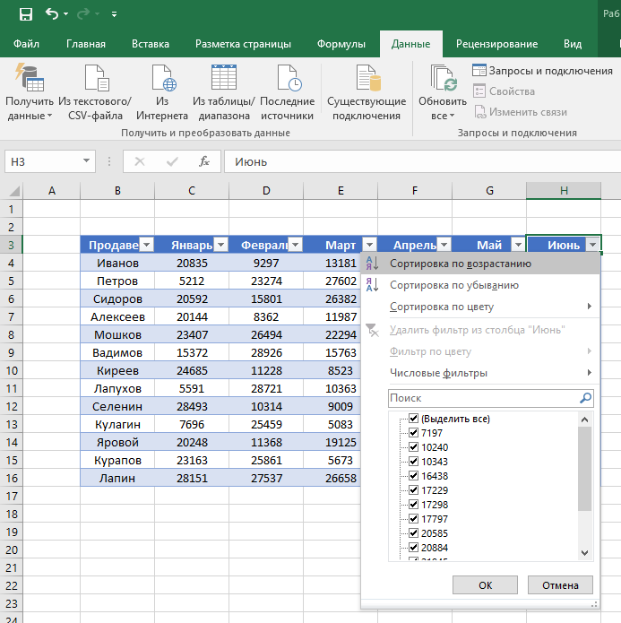
In the window select by what principle to sort the data: “ascending”, “descending”, “by color”, “numerical filters”.

To filter information in the table, click the “arrow” to the right of the column heading, after which a pop-up window will appear:

"Text filter" is displayed when there are text values \u200b\u200bamong the column data; "Filter by color" as well as text filter is available when the table contains cells colored in a color that differs from the standard design; "Numeric filter" allows you to select data by parameters: "Equal … ”,“ Not equal to… ”,“ Greater than… ”,“ Greater than or equal to… ”,“ Less than… ”,“ Less than or equal to… ”,“ Between… ”,“ Top 10 ... ”,“ Above average ”,“ Below average ”, as well as set up your own filter. In the pop-up window, under the“ Search ”all data that can be filtered are displayed, as well as select all values \u200b\u200bor select only empty cells with one click.If you want to undo all created filtering settings, open the pop-up window above the required column again and click “Remove filter from column”. After that, the table will return to its original form.

How to calculate the amount in an Excel spreadsheet

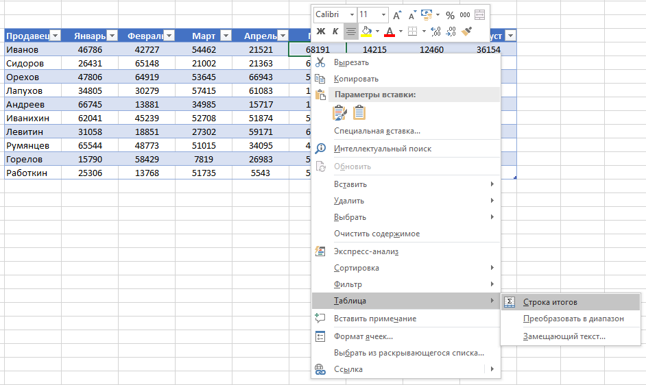
In the window list, select the "Table" \u003d\u003e "Row of totals" item:

A subtotal appears at the bottom of the table. Left-click on the cell with the amount.

In the drop-down menu, select the principle of the subtotal: it can be the sum of the column values, “average”, “quantity”, “number of numbers”, “maximum”, “minimum”, etc.

How to fix the table header in Excel

The tables you have to work with are often large and contain dozens of rows. Scrolling down the table it is difficult to navigate the data if the column headings are not visible. In Excel, it is possible to fix the header in the table in such a way that when you scroll through the data, you will see the column headers.

To freeze headings, do the following:

Go to the "View" tab in the toolbar and select "Freeze Areas":

Select "Freeze Top Row":

Now, scrolling through the table, you will not lose headers and can easily navigate where what data is located:

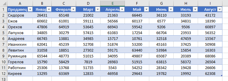
Let's imagine that we have a ready-made table with sales data by manager:

Many of us, regularly faced with financial difficulties, simply do not know how to make a difference. If, unfortunately, you cannot earn more, start spending less! And accounting for the family budget will help you with this. The family budget can be kept in different ways:

keep records in a simple notepad;
keep records on the computer.

There are many different programs that help you manage your family budget. Each family budget planning table, which can be downloaded without problems on the network, has its pros and cons. However, almost all of them are not quite easy to use. Therefore, many people prefer to manage the family budget in Excel. Its main advantages:

it is very simple and convenient;
all income and expenses during the month are clearly displayed in one place;
if Excel's capabilities are not enough, you will already understand what exactly you need, and this will help you find a new program for managing family finances.

How to download and use the family budget spreadsheet in excel?

Plain family budget in excel downloadyou can by clicking on the link at the bottom of the article. Opening the document, you will see 2 sheets:

The first sheet of the family budget planning table records the daily expenses for food and living. Here you can change any cost item to the one that suits you best. The second sheet displays a general report (all cells with formulas are protected from changes. Power expense items are transferred from the first sheet). Here, income and large expenses are also entered: payment of loans, utilities, etc. You can change the sheet by clicking on the corresponding tab at the bottom of the sheet:

Of course, the functionality of such a document is not very great: it does not display statistics of income and expenses, there are no charts and graphs. But, as a rule, those who are looking for it appreciate the simplicity and convenience. After all, the main goal will be achieved: you will begin to really take into account your expenses and compare them with the income you receive. At the same time, having downloaded the family budget in excel, you can print a report on a monthly basis (sizes adjusted to A4 sheet).

How to properly manage your family budget

You need to keep records every day, it will take very little time. All that is needed is to take into account all income and expenses during the day and write down their designated fields. If you have never dealt with keeping a family budget before, then try to force yourself to experiment for 2-3 months. And if you don't like it, then quit. The most important thing in this business is to take into account absolutely all expenses. Large expenses will be remembered very simply, but small ones, on the contrary, are very easy to forget.

It is these small expenses that will amount to 10-30 percent that are spent every month. Try to keep track of all your income and expenses every day. To do this, use all the tools that can help you with this: notebook, check, mobile phone. If you pay attention to spending, you can actually reduce costs. Only for this it is necessary to do something. Start with accounting and your family's wealth will surely increase!