How to make calculations in excel. Creating a calculator in Microsoft Excel

Use for math calculations Microsoft Excel instead of a calculator!

You can enter simple formulas on your worksheet to add, subtract, divide, and multiply two or more numeric values. With the AutoSum feature, you can quickly calculate the sum of a series of values \u200b\u200bwithout manually entering them into a formula. Once you have created a formula once, you can simply place it in adjacent cells without having to create the same formula over and over again.

After you are familiar with these simple formulas, you probably want to know more about creating complex formulas and try out some of the many functions available in Excel. For more information, see Formulas overview and Excel functions by category.

Note: The screenshots in this article were from Excel 2016. Your screens may look different if you are using a different version of Excel.

Simple formulas

All formula entries begin with an equal sign ( = ). To create simple formula, just enter the equal sign followed by the calculated numeric values \u200b\u200band the corresponding math operators: plus sign ( + ) for addition, minus sign ( - ) to subtract, an asterisk ( * ) for multiplication and the slash ( / ) to divide. Then press Enter and Excel will immediately calculate and display the formula result.

For example, if you enter the formula in cell C5 =12,99+16,99 and press Enter, Excel will calculate the result and display 29.98 in that cell.

The formula you enter in a cell will appear in the formula bar whenever you select a cell.

Important: The SUM function exists, but there is no SUBTRACT function. Instead, the formula uses the minus (-) operator. For example: \u003d 8-3 + 2-4 + 12. The minus sign can also be used to convert a number to negative in the SUM function. For example, in the formula \u003d SUM (12; 5; -3; 8; -4), the SUM function adds 5 to 12, subtracts 3, adds 8, and subtracts 4 in that order.

Using AutoSum

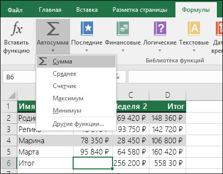
The easiest way to add the SUM formula to a sheet is by using the AutoSum function. Select a blank cell directly above or below the range you want to sum, and then open the ribbon tab home or Formula and select Autosum > Amount... The AutoSum feature automatically determines the range to add and creates a formula. It can also work horizontally if you select a cell to the right or left of the range to be summed.

Note: AutoSum does not work with non-contiguous ranges.

Autosum vertical

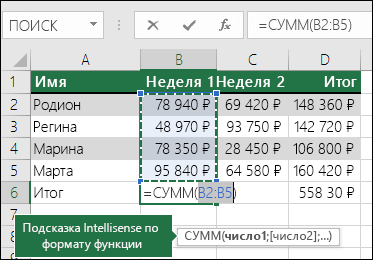
The Auto Sum function automatically identifies cells B2: B5 as the range to sum. You only need to press Enter to confirm. If you need to add or exclude multiple cells, hold down the SHIFT key, press the appropriate arrow key until you select the range you want, and then press Enter.

Intellisense hint for function. The floating tag SUM (number1; [number2];…) below the function is an Intellisense hint. If you click SUM or another function name, it changes to a blue hyperlink that takes you to the Help topic for that function. As you click individual elements of a function, the corresponding portions in the formula are highlighted. In this case, only cells B2: B5 will be selected because there is only one numeric reference in this formula. Intellisense tag appears for any function.

Horizontal AutoSum

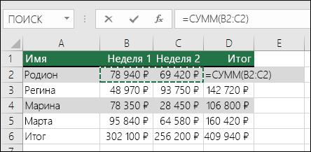
This is not all the summation possibilities! See the article SUM function.

You no longer need to enter a formula multiple times

Once you've created a formula once, you can simply copy it to other cells, rather than creating the same formula over and over. You can copy the formula, or use the fill handle to copy the formula to adjacent cells.

For example, when you copy a formula from cell B6 to cell C6, the cell references in column C are automatically changed.

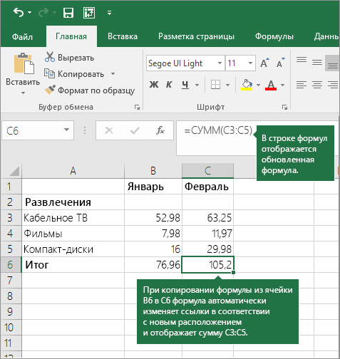
After copying the formula, check that the cell references are correct. Changing cell references depends on their type (absolute or relative). For more information, see the article Copy and paste a formula into another cell or sheet.

What to use in a formula to simulate the keys of a calculator?

Calculator key	Excel method	Description, example	Result
+ (plus key)		Use in a formula to add numbers. Example: \u003d 4 + 6 + 2
- (minus key)		Use in a formula to subtract numbers or indicate a negative number. Example: \u003d 18-12 Example: \u003d 24 * -5 (24 times negative 5)
x (multiply key)	* (asterisk)	Use in a formula to multiply numbers. Example: \u003d 8 * 3
÷ (division key)	/ (slash)	Use in a formula to divide one number by another. Example: \u003d 45/5
% (percent key)	% (percent)	Use * in a formula to multiply by a percentage. Example: \u003d 15% * 20
√ (Square root)	SQRT (function)	Use the SQRT function in a formula to find the square root of a number. Example: \u003d SQRT (64)
1 / x (reciprocal)		Use \u003d 1 / in your formula nwhere n - the number to divide 1 by. Example: \u003d 1/8

Do you have a question about Excel?

Help us improve Excel

Do you have any suggestions for improving the next version of Excel? If so, check out the topics at

Practical work number 20

Performing calculations inExcel

Goal:learn how to perform calculations in Excel

Information from theory

All calculations in MS Excel are performed using formulas. Entering a formula always starts with an equal sign “\u003d”, then the calculated elements are placed, between which there are signs of the operations performed:

+ addition/ division* multiplication

− subtraction^ exponentiation

In formulas, not numbers are often used as operands, but the addresses of the cells in which these numbers are stored. In this case, when you change the number in the cell that is used in the formula, the result will be recalculated automatically

Examples of writing formulas:

\u003d (A5 + B5) / 2

\u003d C6 ^ 2 * (D6- D7)

Formulas use relative, absolute and mixed links to cell addresses. When you copy a formula, relative references change. When copying a formula, the $ sign freezes: the row number (A $ 2 is a mixed reference), the column number ($ F25 is a mixed reference), or both ($ A $ 2 is an absolute reference).

Formulas are dynamic and the results automatically change when the numbers in the selected cells change.

If there are several operations in the formula, then it is necessary to take into account the order of performing mathematical operations.

Autocomplete cells with formulas:

enter the formula in the first cell and press Enter;

select a cell with a formula;

set the mouse pointer to the lower right corner of the cell and drag it in the desired direction (auto-filling of cells with formulas can be done down, up, right, left).

Using functions:

place the cursor in the cell where the calculation will be carried out;

open the list of commands of the Sum button (Fig. 20.1) and select the desired function. When choosing Other functions called Function wizard.

Figure 20.1 - Function selection

Tasks to complete

Task 1 Calculating the dollar rate quotes

In the folder with the name of your group, create an MS Excel document, give the name according to the number of the practical work.

List sheet 1 by the task number;

Create a table for calculating quotations of the dollar rate (Fig.20.2), column the date fill with autocomplete, columns Purchase rateand and Selling rate format as numbers with two decimal places.

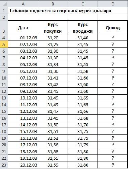
Figure 20.2 - Sample table (Sheet 1)

Perform your income calculation in cell D4. Calculation formula: Income \u003d Selling Rate - Buying Rate

Autocomplete cells D5: D23 with formulas.

In the "Income" column, set Monetary (p) number format;

Format the table.

Save the book.

Task 2 Calculation of total revenue

Sheet 2.

Create a table for calculating the total revenue for the sample, perform the calculations (Fig. 20.3).

In the range B3: E9, specify the currency format with two decimal places.

Calculation formulas:

In total for the day \u003d Branch 1 + Branch 2 + Branch 3;

Total for the week \u003d Sum of values \u200b\u200bfor each column

Format the table. Save the book.

Figure 20.3 - Sample table (Sheet 2)

Task 3 Calculation of the allowance

In the same document go to Sheet 3.Name it by the job number.

Create a table for calculating the allowance for the sample (Fig. 20.4). Column Percentage of markupset format Percentage, set the correct data formats for the columns yourself Salary amountand The amount of the premium.

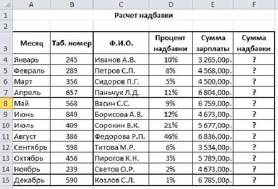
Figure 20.4 - Sample table (Sheet 3)

Perform calculations.

Formula for calculation

Allowance amount \u003d Allowance percentage * Salary amount

After the column Amount surcharges add another column Total... Print in it the total amount of the salary with the bonus.

Enter: in cell E10 Maximum amount of the allowance, into cell E11 - The minimum amount of the premium. To cell E12 - Average amount of the premium.

In cells F10: F12, enter the appropriate formulas for the calculation.

Save the book.

Task 4 Using absolute and relative addresses in formulas

In the same document go to Sheet 4. Name it by the job number.

Enter the table according to the sample (fig.20.5), set the font Bodoni MT,size 12, other formatting settings - according to the sample. For cells C4: C9 set the format Monetary, designation "p.", For cells D4: D9 set the format Monetary, designation "$".

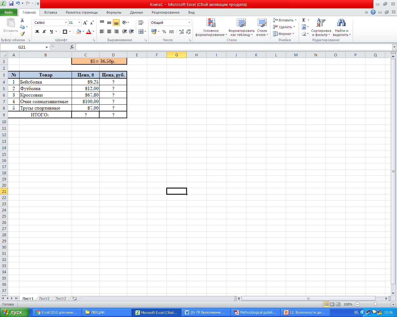
Figure 20.5 - Sample Table (Sheet 4)

Calculate the Values \u200b\u200bof the cells marked with “?”

Save the book.

test questions

How are formulas entered in Excel?

What operations can be used in formulas, how are they indicated?

How do I autocomplete cells with a formula?

How do I call the Function Wizard?

What functions did you use in this practical work?

Tell us how you calculated the values Maximum, Minimumand Average amount of the markup.

How is the cell address formed?

Where in your work did you use absolute addresses, and where - relative?

What data formats did you use in the spreadsheets of this work?

For regular users of Excel, it is no secret that in this program you can perform various mathematical, engineering and financial calculations. This opportunity is realized by using various formulas and functions. But, if Excel is constantly used to carry out such calculations, then the issue of organizing the necessary tools for this directly on the sheet becomes relevant, which will significantly increase the speed of calculations and the level of convenience for the user. Let's find out how to make a similar calculator in Excel.

This task becomes especially urgent, if necessary, to constantly carry out the same type of calculations and calculations associated with a certain type of activity. In general, all calculators in Excel can be divided into two groups: universal (used for general mathematical calculations) and narrow-profile. The latter group is divided into many types: engineering, financial, credit investment, etc. It is the functionality of the calculator that primarily determines the choice of the algorithm for its creation.

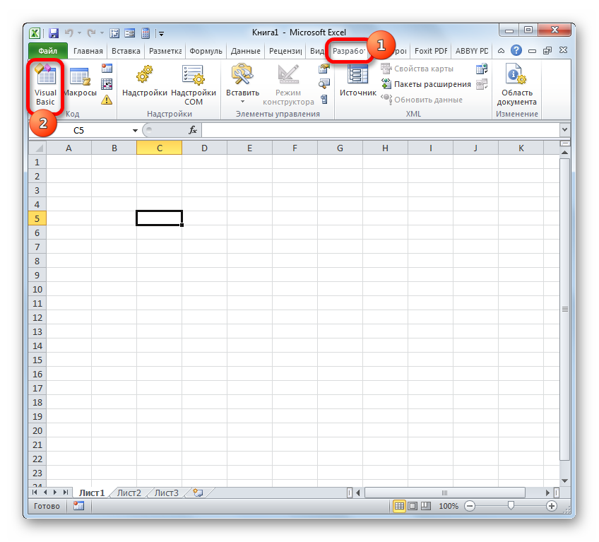
Method 1: using macros

First of all, let's look at the algorithms for creating custom calculators. Let's start by creating the simplest universal calculator. This tool will perform elementary arithmetic operations: addition, multiplication, subtraction, division, etc. It is implemented using a macro. Therefore, before proceeding with the creation procedure, you need to make sure that you have macros and the developer panel enabled. If this is not the case, then you should definitely.

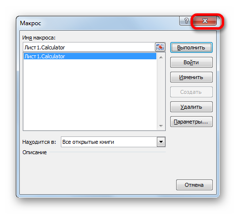
Now, when typing the selected hotkey combination (in our case Ctrl + Shift + V) will launch the calculator window. Agree, this is much faster and easier than calling it through the macro window every time.

Method 2: applying functions

Now let's look at the option of creating a narrow-profile calculator. It will be designed to perform specific, specific tasks and placed directly on excel worksheet... Excel's built-in functions will be used to create this tool.

For example, let's create a tool for converting mass values. In the process of creating it, we will use the function CONVER... This operator belongs to the engineering block of built-in Excel functions. Its task is to convert the values \u200b\u200bof one measure of measurement to another. The syntax for this function is as follows:

CONVER (number; ref_measure; con_ed_measure)

"Number" Is an argument in the form of a numerical value of the quantity that needs to be converted into another measure of measurement.

"Initial unit of measure" - an argument that defines the unit of measurement of the quantity to be converted. It is set by a special code that corresponds to a specific unit of measurement.

"End unit of measure" - an argument defining the unit of measurement of the quantity to which the original number is converted. It is also set using special codes.

We should dwell on these codes in more detail, since we will need them later when creating a calculator. Specifically, we need the codes for the units of measure of mass. Here is a list of them:

g - gram;
kg - kilogram;
mg - milligram;
lbm - British pound;
ozm - ounce;
sg - slag;
u Is an atomic unit.

It should also be said that all the arguments of this function can be set both by values \u200b\u200band by references to the cells where they are located.

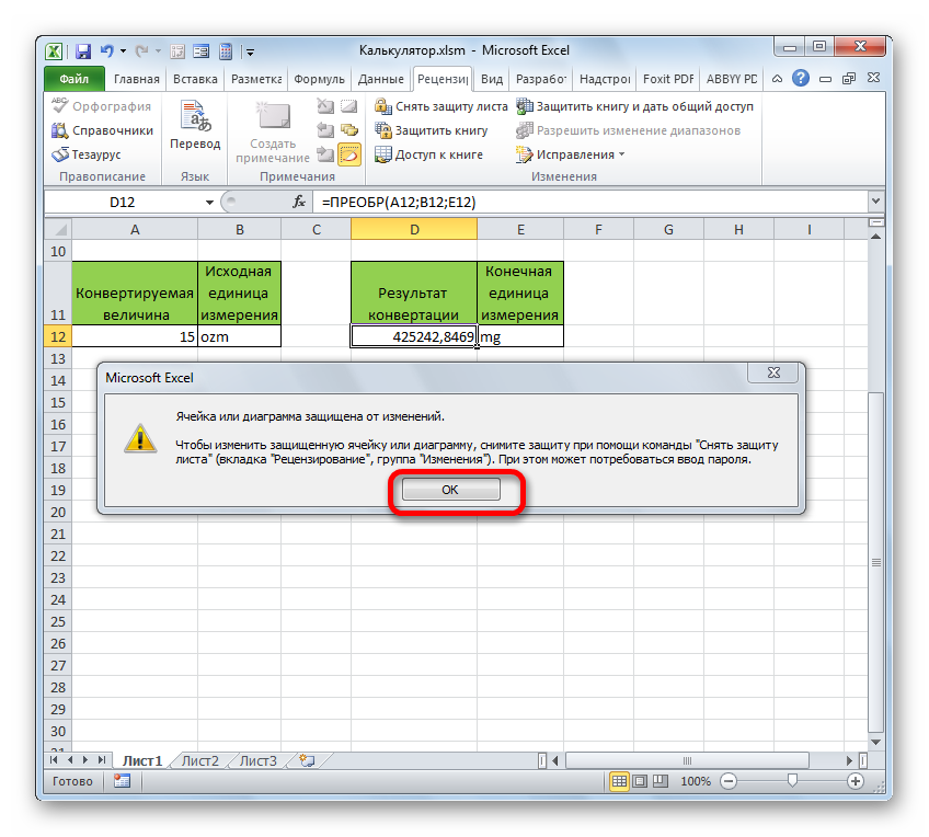
Thus, we have created a full-fledged calculator for converting mass values \u200b\u200binto various units of measurement.

In addition, a separate article tells about the creation of another type of narrow-profile calculator in Excel for calculating loan payments.

Use for math microsoft computing Excel instead of a calculator!

Once you are familiar with these simple formulas, you will probably want to learn more about creating complex formulas and try some of the many functions available in Excel. For more information, see Formulas overview and Excel functions by category.

Note: The screenshots in this article were from Excel 2016. Your screens may look different if you are using a different version of Excel.

Simple formulas

All formula entries begin with an equal sign ( = ). To create a simple formula, simply enter an equal sign followed by the calculated numeric values \u200b\u200band the corresponding math operators: the plus sign ( + ) for addition, minus sign ( - ) to subtract, an asterisk ( * ) for multiplication and the slash ( / ) to divide. Then press Enter and Excel will immediately calculate and display the formula result.

For example, if you enter the formula in cell C5 =12,99+16,99 and press Enter, Excel will calculate the result and display 29.98 in that cell.

The formula you enter in a cell will appear in the formula bar whenever you select a cell.

Using AutoSum

Note: AutoSum does not work with non-contiguous ranges.

Autosum vertical

Horizontal AutoSum

This is not all the summation possibilities! See the article SUM function.

You no longer need to enter a formula multiple times

For example, when you copy a formula from cell B6 to cell C6, the cell references in column C are automatically changed.

What to use in a formula to simulate the keys of a calculator?

Calculator key	Excel method	Description, example	Result
+ (plus key)		Use in a formula to add numbers. Example: \u003d 4 + 6 + 2
- (minus key)		Use in a formula to subtract numbers or indicate a negative number. Example: \u003d 18-12 Example: \u003d 24 * -5 (24 times negative 5)
x (multiply key)	* (asterisk)	Use in a formula to multiply numbers. Example: \u003d 8 * 3
÷ (division key)	/ (slash)	Use in a formula to divide one number by another. Example: \u003d 45/5
% (percent key)	% (percent)	Use * in a formula to multiply by a percentage. Example: \u003d 15% * 20
√ (Square root)	SQRT (function)	Use the SQRT function in a formula to find the square root of a number. Example: \u003d SQRT (64)
1 / x (reciprocal)		Use \u003d 1 / in your formula nwhere n - the number to divide 1 by. Example: \u003d 1/8

Do you have a question about Excel?

Help us improve Excel

Do you have any suggestions for improving the next version of Excel? If so, check out the topics at