Problems with calculating formulas in Microsoft Excel. Page mode of worksheet in Excel. Information in comments

One of the most requested features of Excel is working with formulas. Thanks to this function, the program independently performs various kinds of calculations in tables. But sometimes it happens that the user enters a formula into a cell, but it does not fulfill its direct purpose - to calculate the result. Let's figure out what this may be related to, and how to solve this problem.

The reasons for problems with the calculation of formulas in Excel can be completely different. They can be caused both by the settings of a particular book or even a separate range of cells, or by various errors in syntax.

Method 1: change the format of cells

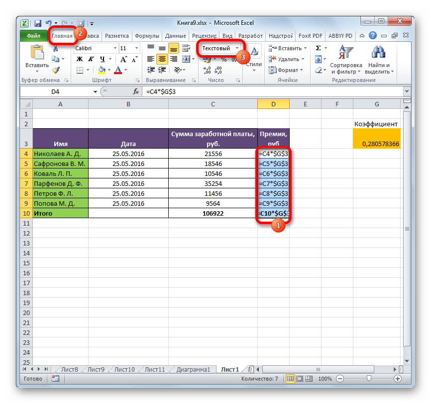
One of the most common reasons why Excel does not calculate at all or does not calculate formulas correctly is the incorrectly set format of cells. If the range has text format, then the calculation of expressions in it is not performed at all, that is, they are displayed as ordinary text. In other cases, if the format does not correspond to the essence of the calculated data, the result displayed in the cell may be displayed incorrectly. Let's find out how to fix this problem.

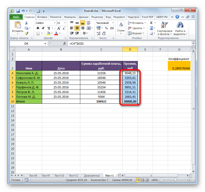
Now the formula will be calculated in the standard order with the output of the result in the specified cell.

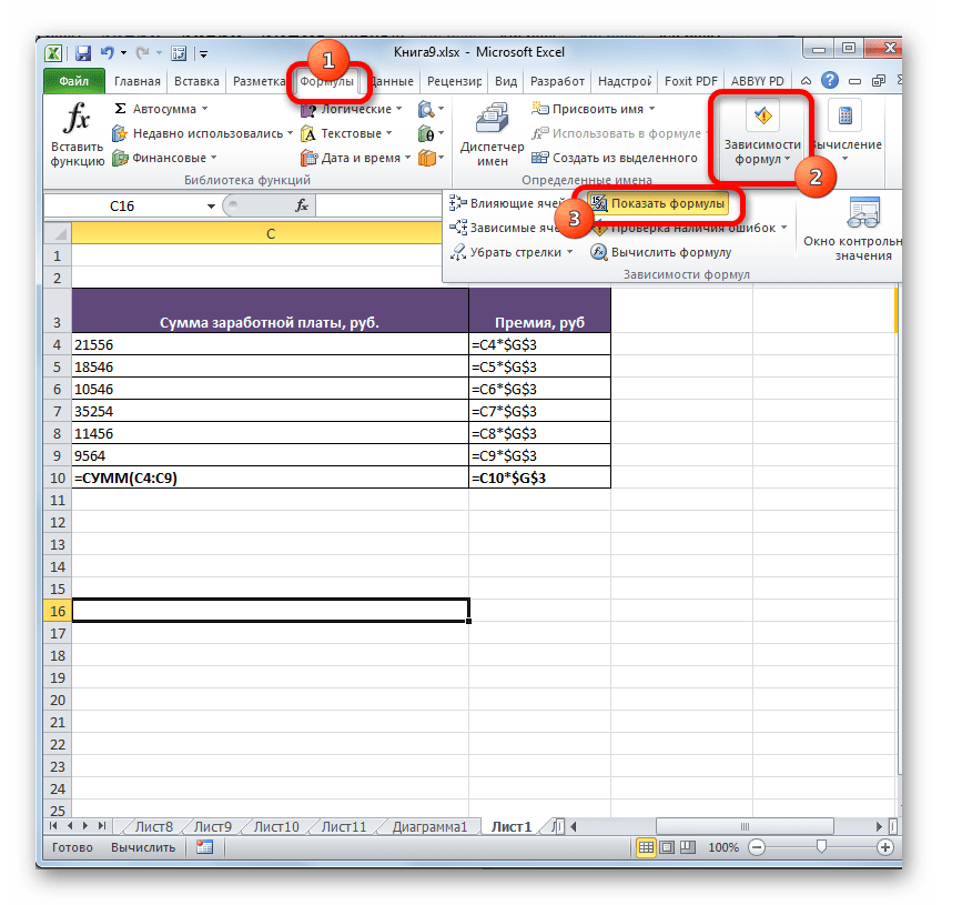
Method 2: turn off the "Show formulas" mode

But perhaps the reason that instead of the calculation results you display expressions is that the program has enabled the mode "Show formulas".

Method 3: fix a syntax error

A formula can also be displayed as text if errors were made in its syntax, for example, a letter was missing or changed. If you entered it manually, and not through Function wizard, then this is quite likely. A very common mistake when displaying an expression as text is the presence of a space before the sign «=» .

In such cases, you need to carefully review the syntax of those formulas that are displayed incorrectly, and make the appropriate adjustments.

Method 4: enable formula recalculation

It also happens that the formula seems to display the value, but when the cells associated with it change, it does not change itself, that is, the result is not recalculated. This means that you have misconfigured the calculation parameters in this book.

All expressions in this workbook will now be automatically recalculated whenever any associated value changes.

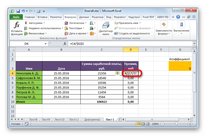
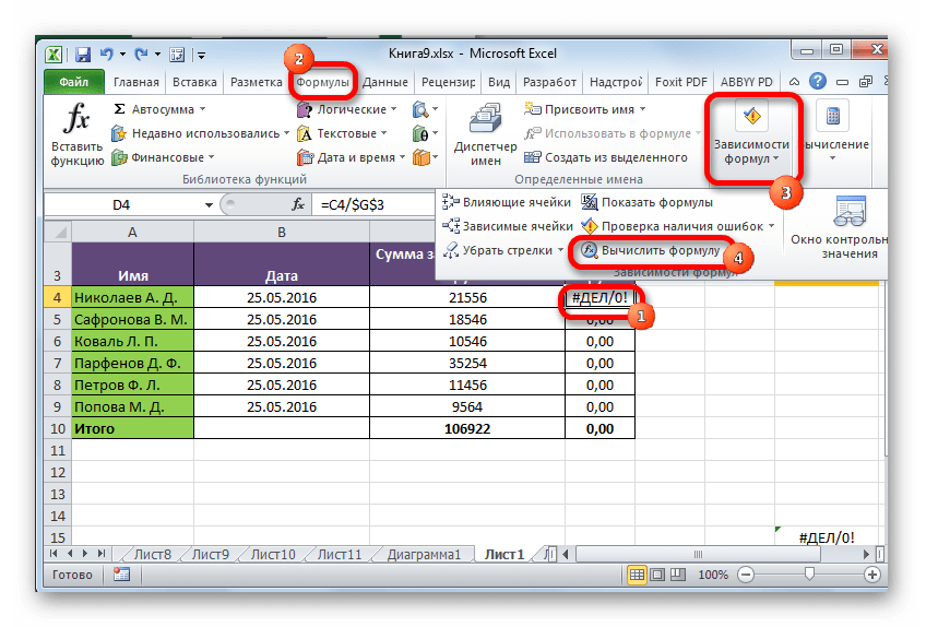
Method 5: error in the formula

If the program still calculates, but as a result shows an error, then it is likely that the user simply made a mistake when entering the expression. Erroneous formulas are those, when calculating which the following values appear in the cell:

#NUMBER!;
#VALUE !;
# EMPTY !;
# DIV / 0 !;
# N / A.

In this case, you need to check whether the data in the cells referenced by the expression is correctly written, whether there are any syntax errors or whether the formula itself contains any incorrect action (for example, division by 0).

If the function is complex, with a large number of linked cells, it is easier to trace the calculations using a special tool.

As you can see, the reasons why Excel does not consider or does not correctly calculate the formulas can be completely different. If, instead of calculating, the user displays the function itself, then in this case, most likely, either the cell is formatted for text, or the expression view mode is enabled. Also, a syntax error is possible (for example, the presence of a space before the sign «=» ). If, after changing the data in the linked cells, the result is not updated, then here you need to see how auto-update is configured in the book parameters. Also, quite often, instead of the correct result, an error is displayed in the cell. Here you need to view all the values that the function refers to. If an error is found, it should be eliminated.

Lifehacker readers are already familiar with Denis Batyanov who shared with us. Today Denis will talk about how to avoid the most common problems with Excel, which we often create for ourselves.

I'll make a reservation right away that the article material is intended for beginner Excel users. Experienced users have already danced incendiaryly on this rake more than once, so my task is to protect young and inexperienced "dancers" from this.

You do not give titles to table columns

Many Excel tools, such as sorting, filtering, smart tables, pivot tables, assume that your data contains column headers. Otherwise, you will either not be able to use them at all, or they will not work quite correctly. Always make sure your tables contain column headings.

Empty columns and rows inside your tables

This is confusing for Excel. Upon encountering an empty row or column inside your table, it starts thinking that you have 2 tables, not one. You will have to constantly correct it. Also, do not hide the rows / columns you do not need inside the table, it is better to delete them.

Several tables are located on one sheet

If these are not tiny tables containing reference values, then you should not do this.

It will be inconvenient for you to fully work with more than one table per sheet. For example, if one table is on the left and the second on the right, then filtering on one table will affect the other. If the tables are located one below the other, then it is impossible to use the pinning of areas, and one of the tables will have to constantly search and perform unnecessary manipulations in order to stand on it with a table cursor. Do you need it?

Data of the same type is artificially arranged in different columns

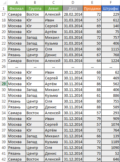
Very often, users who know Excel rather superficially prefer this table format:

It would seem that we are faced with a harmless format for accumulating information on the sales of agents and their fines. Such a table layout is well perceived by a person visually, since it is compact. However, believe me, it is a real nightmare to try to extract data from such tables and get subtotals (aggregate information).

The fact is that this format contains 2 dimensions: so that you have to decide on the line by going through the branch, group and agent. When you find the right stock, then you will have to search for the required column, since there are a lot of them here. And this "two-dimensionality" greatly complicates the work with such a table for standard Excel tools - formulas and pivot tables.

If you build a pivot table, you will find that there is no way to easily get the data by year or quarter, since the indicators are split into different fields. You do not have one sales field that can be conveniently manipulated, but there are 12 separate fields. You will have to create by hand separate calculated fields for quarters and years, although, be it all in one column, pivot table would do it for you.

If you want to apply standard summation formulas like SUMIF, SUMIFS, SUMPRODUCT, you will also find that they will not work effectively with this table layout.

Distribution of information on different sheets of the book "for convenience"

Another common mistake is, having some kind of standard table format and needing analytics based on this data, distribute it to separate sheets of the Excel workbook. For example, they often create separate sheets for each month or year. As a result, the amount of data analysis work is actually multiplied by the number of sheets created. Don't do that. Collect information on ONE sheet.

Information in comments

Often users add important information they may need in the cell comment. Keep in mind that what is in the comments, you can only look (if you find it). Pulling this out into the cell is difficult. I recommend it is better to have a separate column for comments.

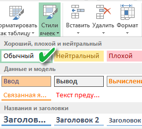
A mess with formatting

Definitely won't add any good to your table. This looks off-putting to people using your spreadsheets. At best, they will not attach importance to this, at worst - they will think that you are not organized and sloppy in business. Strive for the following:

Merging cells

Use cell concatenation only when you can't do without it. Merged cells make it very difficult to manipulate the ranges they fall into. Problems occur when moving cells, inserting cells, etc.

Combine text and numbers in one cell

A painful impression is produced by a cell containing a number, padded behind by the text constant "RUB." or "USD" entered manually. Especially if it is not a printed form, but a regular table. Arithmetic operations with such cells are naturally impossible.

Numbers as text in a cell

Avoid storing numeric data in a cell in text format. Over time, some of the cells in such a column will have a text format, and some will have a regular one. There will be problems with formulas because of this.

If your table will be presented through an LCD projector

Choose the most contrasting combinations of color and background. Looks good on a projector dark background and light letters. The most terrible impression is made by red on black and vice versa. This combination looks extremely low-contrast on the projector - avoid it.

Page mode worksheet in Excel

This is the same mode in which Excel shows how the sheet will be paginated when printed. Page borders are highlighted in blue. I do not recommend constantly working in this mode, which many do, since the printer driver is involved in the process of displaying data on the screen, and this, depending on many reasons (for example, a network printer is not available at the moment), is fraught with freezes in the rendering process and recalculating formulas. Work as usual.

For even more useful information about Excel, visit

Often enough data from third-party programs is downloaded to Excel for their further processing, and often further use of this data in formulas gives an unpredictable result: numbers are not summed up, it is impossible to calculate the number of days between dates, etc.

This article discusses the causes of such problems and different ways their elimination

Reason one ... Number saved as text

In this case, you can see that numbers or dates are pressed to the left edge of the cell (as text) and, as a rule, in the upper left corner of the cell there is an error marker (green triangle) and a tag that, when you hover the mouse, explains that the number is saved as text.

No changes in the format to Numeric, General or Date do not correct the situation, but if you click in the formula bar (or press F2) and then Enter, the number becomes a number, and the date becomes a date. With a large number of such numbers, the option, you see, is unacceptable.

There are several ways to solve this problem.

Using an error marker and tag... If you see an error marker ( green triangle) and tag, then select the cells, click on the tag and select the option Convert to number

Using the Find / Replace operation... Suppose there are numbers with a decimal point in the table, stored as text. Select a range with numbers - click Ctrl + h(or find on the tab home or on the menu Edit for versions prior to 2007 the command Replace) -- in field Find introduce , (comma) - in the field Replaced by we also introduce , (comma) - Replace all... Thus, by replacing comma with comma, we simulate cell editing in the same way F2 - Enter

A similar operation can be performed with dates, with the only difference that you need to change point to point.

In addition, third-party programs can unload numbers with a dot as a decimal separator, then replacing a dot with a comma will help.

A similar replacement can be done with the formula (see below) using the SUBSTITUTE () function

Using Paste Special... This method is more versatile, as it works with fractional numbers, integers, and dates. Select any empty cell - execute the command Copy- select the range with problem numbers - Paste special -- To fold-- OK... Thus, we add 0 to numbers (or dates), which does not affect their value in any way, but converts to a number format

A variation of this technique could be to multiply the range by 1

Using the Text by Columns tool... This technique is convenient to use if you need to transform one column, since if there are several columns, then the steps will have to be repeated for each column separately. So, select the column with numbers or dates saved as text, set the cell format General(for numbers, you can set, for example, Numerical or Financial). Next, we execute the command Data-- Column Text -- Ready

Using formulas... If the table allows additional columns, you can use formulas to convert to a number. To convert a text value to a number, you can use double minus, addition with zero, multiplication by one, the VALUE (), SUBSTITUTE () functions. You can read in more detail. After transformation, the resulting column can be copied and pasted as values in place of the original data

By using... Actually, any of the listed methods can be performed with a macro. If you have to do this kind of conversion often, then it makes sense to write a macro and run it as needed.

Here are two examples of macros:

1) multiply by 1

Sub conv () Dim c As Range For Each c In Selection If IsNumeric (c.Value) Then c.Value = c.Value * 1 c.NumberFormat = "#, ## 0.00" End If Next End Sub

2) text by columns

Sub conv1 () Selection.TextToColumns Selection.NumberFormat = "#, ## 0.00" End Sub

Reason two ... The number contains extraneous characters.

Most often, these extraneous characters are spaces. They can be located both inside the number as a separator of digits, and before / after the number. In this case, naturally, the number becomes text.

Put away extra spaces can also be done using the operation Find / Replace... In field Find enter a space, and the field Replaced by leave blank, then Replace all... If there were ordinary spaces in the number, then these actions will be enough. But the number may contain the so-called non-breaking spaces (symbol with code 160). Such a space will have to be copied directly from the cell, and then pasted into the field Find dialog box Find / Replace... Or you can in the field Find press the keyboard shortcut Alt + 0160(numbers are typed on the numeric keypad).

Spaces can also be removed with a formula. The options are:

For regular spaces: = - SUBSTITUTE (B4; ""; "")

For non-breaking spaces:= - SUBSTITUTE (B4, SYMBOL (160), "")

Immediately for those and other spaces: = - SUBSTITUTE (SUBSTITUTE (B4; SYMBOL (160); ""); ""; "")

Sometimes, in order to achieve the desired result, you have to combine the listed methods. For example, remove spaces first and then convert cell format