Pivot table items. What will we do with the received material. Show and hide detail data

The main elements of pivot tables. Before continuing this work, I think it would not be superfluous to tell what elements pivot tables are made of, and for this, consider the example in Figure 2. A page field is a field in the original list or table placed in the page orientation area pivot table.

In this example, Scope is a page margin that can be used to summarize by region. When you specify another page field item, the pivot table is recalculated to display the totals associated with that item. Page field value - Page field elements combine the records or values \u200b\u200bof a field or column in the original list of the table. In other words, this is by switching this field, in fact, every time there is a transition to a new data source for a new region.

Row fields are fields in the original list or table that have been placed in the row area of \u200b\u200bthe PivotTable. In this example, Products and Vendor are string fields. Internal row fields for example Salesperson exactly match the data area external row fields for example Products group internal ones. Thus, a certain rule is traced here, each element of a higher level field, as it were, perfects all fields of a lower level, the product parameter limits all data under it - product sellers, data on product sales by these sellers. A column field is a field in a source list or table that is placed in the column area.

In this example, Quarters is a column field that includes two field elements KB2 and KB3. The inner fields of the columns contain elements, the corresponding data areas are the outer fields of the columns located above the inner fields. The example shows only one column field.

A data area is the portion of a PivotTable that contains the totals. Data area cells display totals for row or column field items. The values \u200b\u200bin each cell of the data area correspond to the original data. In this example, cell C6 summarizes all raw data records containing the same product name, distributor, and a specific quarter Meat, Myastorg LLP, and KB2. Field items are subcategories of a PivotTable field. In this example, the values \u200b\u200bMeat and Seafood are field items in the Products field.

Field items represent records in a field or column in the source data. Field items appear as row or column headings, and in the drop-down list for page fields. A data field is a field in a source list or table that contains data. In this example, the Order Amount field is a data field that summarizes the original data in the Order Amount field or column. A data field usually summarizes a group of numbers such as statistics or sales quantities, although the current data can also be textual.

By default, a PivotTable summarizes text data using the Total Values \u200b\u200bsummary function, and numerical data using the Sum summary function. Changing the structure of a pivot table Appearance You can edit the pivot table directly on the sheet by dragging the names of field buttons or field items. You can also change the order of the elements in the field, for which you need to select the element name, and then set the pointer to the cell border.

When the pointer changes to an arrow, drag the field cell to a new location. To remove a field, drag the field button outside the details area. Deleting a field will hide all dependent values \u200b\u200bin the pivot table, but will not affect the original data. If you need to use all the provided tools for structuring the pivot table, or if the current table has not previously included all the fields of the source data, you should use the pivot table wizard.

If the pivot table contains a large group of page fields, then they can be placed in rows or columns. In addition, it should be noted that changing the structure of the PivotTable does not affect the original data.

End of work -

This topic belongs to the section:

Processing tabular information using pivot tables using Microsoft Excel

By swapping rows and columns, you can create new totals of the original data by displaying different pages you can filter the data, and ... In other words, these tables allow you to combine data from different sources, ... Creating a pivot table Before creating a pivot table, you must first set the data for this table, ...

If you need additional material on this topic, or you did not find what you were looking for, we recommend using the search in our work base:

What will we do with the received material:

If this material turned out to be useful for you, you can save it to your page on social networks:

All topics in this section:

Creating a pivot table
Create a pivot table. Before creating a pivot table, you must first set the data for this table by selecting part of the book, pages, and if it is a database or a list, then n

PivotTable Details and Actions
The details of the pivot table and the actions performed on it. Detail data is a subcategory of a pivot table. These pivot table items are unique table items or with

Show or hide detailed PivotTable data
Show or hide detailed pivot table data. In order to display detailed data that was previously hidden, or hide existing data, you need to select the field element, detailed data

Show or hide PivotTable field items
Show or hide PivotTable field items. If you need to display or hide a field element, then for this you must, first, select the field in which you want to display or

Display maximum or minimum items in a pivot table field
Displays the maximum or minimum items in a PivotTable field. To display the maximum or minimum elements, it is necessary to select the field in which the elements will be shown in the future.

Disable access to pivot table details
Disable access to pivot table details. If you position the pointer over a cell in the data area of \u200b\u200ba PivotTable and double-click, a summary list of the source data is displayed

Grouping and ungrouping data in a pivot table
Grouping and ungrouping data in a pivot table. In a pivot table, you can group dates, times, numbers, and selected items. For example, you can combine months to summarize the sq.

Group and ungroup items in a PivotTable field
Group and ungroup items in a PivotTable field. To group and ungroup elements, you need to select the grouped elements. Then click the Group button on the panel

Group and ungroup numbers in a pivot table
Group and ungroup numbers in a pivot table. To group and ungroup numbers, select the number in the box where you want to group the items. Then press the button

Group and ungroup dates or times in a pivot table
Group and ungroup dates or times in a pivot table. To group and ungroup a date or time, select the date or time in the field in which to group the item.

Group and Ungroup Pivot Table Page Field Items
Group and ungroup the elements of a PivotTable page field. If the pivot table is created from an external data source, check that the page field is fetching external data

Refresh or change the data source of the pivot table. In the process of work, sometimes a situation arises when new data appears that must be inserted into the created document, and

Refreshing data in a pivot table
Refresh data in a pivot table. In order to update the data in the pivot table, you need to do the following operations.It is necessary to select the cell in the pivot table, the content of which is required

Disable pivot table refresh when opening workbook file
Disable refreshing the pivot table when opening a workbook file. To disable refreshing the pivot table when opening a file, select a cell in the pivot table for which no refresh will occur

Sorting pivot table data
Sorting pivot table data. PivotTable field items are automatically sorted in ascending order according to their name. Sorting items by name allows you to restore the original

Summarizing and processing pivot table data
Summing up and processing the data of the pivot table. Pivot table data fields can be configured for calculations other than the default in the summary function. To perform complex

Using grand totals and subtotals in a pivot table
Using grand totals and subtotals in a pivot table. A PivotTable can be configured to perform calculations using a summary function. A summary function is the type of calculation performed by

Insert or remove subtotals in a pivot table
Insert or remove subtotals in a pivot table. In order to insert or delete subtotals, you need to set the pointer to the button of the field in which you want to

Create a chart for a pivot table
Create a chart for a pivot table. To create a chart for a pivot table, on the PivotTables toolbar, select the Select command from the PivotTable menu. Check that

This post introduces a collection of simple and nifty PivotTable tools in Excel. What is called tips & tricks in English. Take the time to read the tips here. Who knows, maybe you will finally find the answer to the question that has tormented you for a long time?

Tip 1. Automatic refresh of pivot tables

Sometimes you want pivot tables to update automatically. Let's say you've created a pivot table for a manager. It is unlikely that you will be able to regularly update it, unless the manager will let you to his laptop. You can enable automatic update a pivot table to run whenever the workbook is opened:

1. Right-click on the PivotTable and select Pivot table options.
2. In the dialog box that appears Pivot table options select tab Data.
3. Check the box Refresh on file open.

Figure: 1. Enable the option Refresh on file open

Checkbox Refresh on file open should be installed for each pivot table separately.

Download the note in the format or, examples in the format (the file contains the VBA code).

Tip 2: Simultaneously update all pivot tables in a book

If a workbook contains multiple pivot tables, updating them at the same time can be problematic. There are several ways to overcome these difficulties:

Method 1. For each pivot table included in the workbook, you can select a setting that automatically refreshes when the workbook is opened (for more information, see Tip 1).

Method 3: Use VBA code to update all pivot tables in the workbook on demand. This approach uses the RefreshAll method of the Workbook object. To use this technique, create a new module and enter the following code:

Sub Refresh_All ()

ThisWorkbook.RefreshAll

Tip 3. Sort items in random order

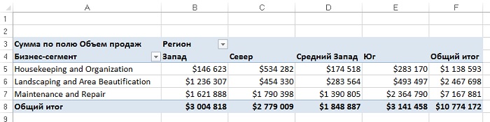
In fig. Figure 2 shows the default display order of regions in a PivotTable. Regions are sorted in alphabetical order: West, North, Midwest, and South. If your corporate rules require you to display the West region first and then the Midwest, North, and South regions, do a manual sort. Just enter Midwest into cell C4 and press the key Enter... The sort order of regions will change.

Tip 4: Convert PivotTable to Hardcoded Values

The purpose of creating a pivot table is to summarize and display data in suitable format... The original data for the PivotTable is stored separately, which introduces some "overhead". Converting the pivot table to values \u200b\u200bwill allow you to use the results obtained in it without accessing the original data or the pivot table cache. How the pivot table is transformed depends on whether the entire table is affected or only part of it.

To convert part of a PivotTable, follow these steps:

1. Select the copied PivotTable data, right-click and select Copy (or type Ctrl + C on your keyboard).
2. Right-click anywhere on the worksheet and select the command Paste (or type Ctrl + V).

If you need to convert the entire PivotTable, follow these steps:

1. Select the entire PivotTable, right-click and select Copy... If the PivotTable does not contain the FILTERS area, you can use the Ctrl + Shift + * keyboard shortcut to select the PivotTable area.
2. Right-click anywhere on the sheet and select an option from the context menu Paste special.
3. Select an option The values and click OK.

It is a good idea to delete the subtotals before converting the PivotTable because they are not very useful in the offline dataset. To delete all subtotals, go to the Design menu -\u003e Subtotals -\u003e Do not show subtotals. To delete specific subtotals, right-click the cell in which the totals are calculated. Select the item in the context menu Field parameters and in the dialog Field parameters in section Outcome select radio button Not... After clicking the button OK subtotals will be deleted.

Tip 5. Filling empty cells in the LINE fields

After converting the PivotTable, the sheet displays not only the values, but the entire data structure of the PivotTable. For example, the data shown in Fig. 3 were derived from a pivot table with a tabular layout.

Figure: 3. It is problematic to use this converted pivot table without filling in empty cells on the left side

Note that the fields Region and Sales market maintains the same row structure as when this data is found in the ROWS area of \u200b\u200ba pivot table. Excel 2013 has quick way filling the cells in the LINE area with values. Click in the pivot table area, then go through the menu Constructor -> Report layout -> (fig. 4). You can then convert the pivot table to values, which will give you a data table with no spaces.

Figure: 4. After applying the command Repeat all item labels all empty cells are filled

Tip 6: Ranking numeric fields in a pivot table

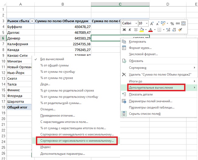
In the process of sorting and ranking fields containing a large number of data items, it is not always easy to determine the numerical rank of the data item being analyzed. Moreover, if the pivot table is converted to values, assigning each data item a numeric rank displayed in an integer field will greatly facilitate analysis of the generated dataset. Open a pivot table like the one shown in Fig. 5. Note that the same indicator - Amount by field Sales volume - displayed twice. Right-click on the second instance of the metric and select the command Additional calculations -> Sorting from maximum to minimum (fig. 6.)

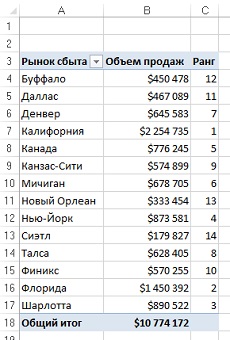
After creating a rank, you can customize the field captions and formatting (Figure 14.9). The result will be a nice ranked report.

Tip 7: Reduce the size of a PivotTable report

When you generate a PivotTable report, Excel takes a snapshot of the data and stores it in the PivotTable cache. The pivot table cache is a special area of \u200b\u200bmemory that stores a copy of the data source to speed up access. In other words, Excel creates a copy of the data and then stores it in a cache associated with the workbook. The pivot table cache provides workflow optimization. Any changes made to the PivotTable, such as changing the layout of fields, adding new fields, or hiding items, are faster, and the system resource requirements are much more modest. The main disadvantage of PivotTable Cache is that it nearly doubles the size of the workbook file each time a PivotTable is created from scratch.

Delete the original data.If the workbook contains an original dataset and a pivot table, its file size is doubled. Therefore, you can safely delete the original data, and this will not affect the functionality of your pivot table at all. After deleting the original data, remember to save the compressed version of the workbook file. After deleting the original data, you can use the pivot table as usual. The only problem is the inability to update the pivot table due to the lack of original data. If you need some background data, double-click the intersection of the row and column in the grand totals area (in Figure 7, this is cell B18). In doing so, Excel dumps the contents of the pivot table cache into a new worksheet.

Tip 8: Create an auto-expandable data range

Surely you have repeatedly encountered situations when you had to update PivotTable reports on a daily basis. This is most often needed when new records are constantly being added to the data source. In such cases, you will have to redefine the previously used range before the new records are added to the new PivotTable. Redefining the original data range for a PivotTable is easy, but when you do it often, it becomes quite tedious.

The solution to the problem is to convert the original data range to a table even before the pivot table is created. Thanks to excel spreadsheets you can create a named range that can automatically expand or contract depending on the amount of data in it. You can also link any component, chart, PivotTable, or formula to a range so that you can track changes in the dataset.

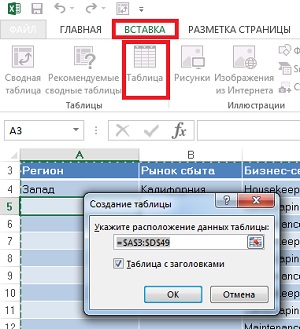
To implement the described technique, select the source data, and then click on the table icon located on the tab Insert (fig. 8) or press Ctrl + T (English T). Click OK in the window that opens. Note that although you do not need to redefine the source data range in the pivot table, you will still have to click the button when you add source data to the range in the pivot table. Refresh.

Tip 9: Compare regular tables with a pivot table

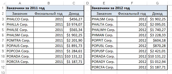
If you are comparing two different tables, it is convenient to use a pivot table, which will save you a lot of time. Suppose you have two tables that display customer details for 2011 and 2012 (Figure 9). The small dimensions of these tables are given here solely as examples. In practice, tables are used that are much larger.

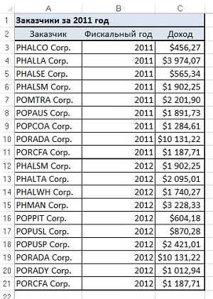
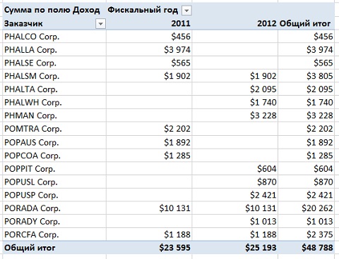
The comparison creates a single table from which a pivot table is created. Make sure you have a way to tag the data related to these tables. In this example, this uses the column Fiscal year (fig. 10). After combining the two tables, use the resulting combined dataset to create a new PivotTable. Format the PivotTable so that the PivotTable Column area is used as the table tag (an identifier that indicates the origin of the table). As shown in fig. 11, years are in the column area and customer details are in the row area. The data area contains the sales volumes for each customer.

Tip 10: Automatic filtering of a pivot table

As you know, autofilters cannot be applied to pivot tables. However, there is a trick to enable AutoFilters in a PivotTable. The principle behind this technique is to place the mouse pointer to the right of the last header of the PivotTable (cell D3 in Figure 12), then go to the ribbon and select Data -> Filter... From now on, an autofilter appears in your pivot table! For example, you can select all customers with a higher than average transaction rate. AutoFilters add an extra layer of analytics to the PivotTable.

Tip 11. Convert datasets displayed in pivot tables

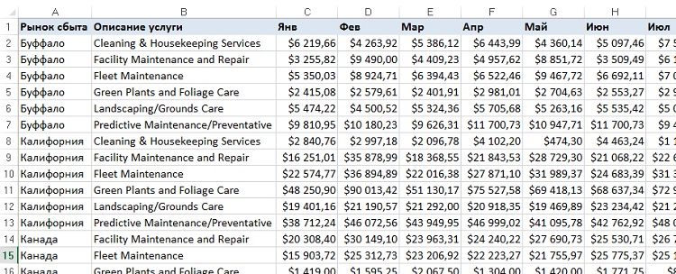
The best layout for the original data converted to a PivotTable is the tabular layout. This type of layout has the following features: there are no empty rows or columns, each column has a header, each field has a value in each row, and the columns do not contain duplicate data groups. In practice, there are often datasets that resemble the one shown in Fig. 13. As you can see, the month names are displayed in a row along the top of the table, performing the dual function of column labels and actual data. In a pivot table created from such a table, this would result in 12 fields to manage, each representing a separate month.

To eliminate this problem, you can use a pivot table with several consolidated ranges as an intermediate step (see details). To convert a dataset that has a matrix style to a dataset that is more suitable for creating pivot tables, follow these steps.

Step 1. Combine all non-columnar fields into one column.To create pivot tables with multiple consolidated ranges, create a single dimension column. In this example, everything that is not related to the month field is considered as a dimension. Therefore the fields Sales market and Service description should be merged into one column. To combine fields into one column, simply enter a formula that concatenates the two fields using a semicolon as a separator. Give the new column a name. The entered formula is displayed in the formula bar (Fig. 14).

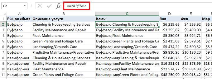
Figure: 14. Result of column concatenation Sales market and Service description

After creating the concatenated column, convert formulas to values. To do this, select the newly created column, press Ctrl + C, and then run the command Paste -> Paste special -> The values... Columns can now be removed Sales market and Service description (fig. 15).

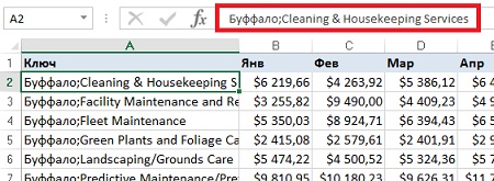
Figure: 15. Deleted columns Sales market and Service description

Step 2. Create a pivot table with multiple consolidation ranges.Now you need to call the PivotTable and Chart Wizard familiar to many users from previous versions of Excel. Press Alt + D + P to invoke this wizard. Unfortunately, this keyboard shortcut is for the English version of Excel 2013. In the Russian version, it corresponds to the keyboard shortcut Alt + D + N. But it doesn't work for reasons unknown to me. However, you can bring the good old PivotTable Wizard to the Quick Access Toolbar, see. After starting the wizard, select the radio button In multiple ranges of consolidation... Click Further... Set the switch Create page fields and click Further... Define the working range and click Done (see details). You will create a pivot table (Figure 16).

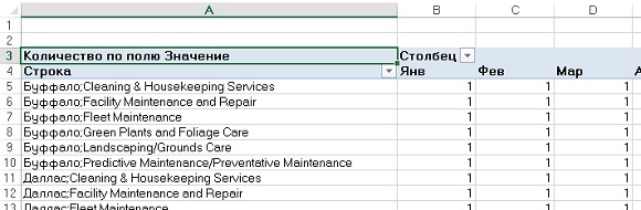
Step 3. Double-click the intersection of a row and a column in the grand total row.At this point, you will have a pivot table (Figure 16) that includes several consolidation ranges, which is almost useless. Select the cell that is at the intersection of the row and the grand total column and double-click on it (in our example, this is cell N88). You will get a new sheet with a structure similar to the one shown in Fig. 17. In fact, this sheet is a transposed version of the original data.

Step 4. Splitting the Row column into separate fields.It remains to split the column Line into separate fields (return to the original structure). Add one empty column immediately after the column Line... Highlight column A and then go to the ribbon tab Data and click on the button Column Text... A dialog box appears on the screen Text Distribution Wizard... In the first step, select the radio button Delimitedand click the Next button. In the next step, select the radio button semicolon and click Done... Format the text, add a title and turn the original data into a table by pressing Ctrl + T (Figure 18).

Figure: 18. This dataset is ideal for creating a pivot table (compare with Fig. 13)

Tip 12: Include two number formats in a pivot table

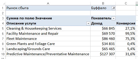
Now consider a situation where a normalized dataset makes it difficult to build a pivot table that is easy to analyze. An example is shown in Fig. 19 is a table that includes two different indicators for each sales area. Notice column D, which identifies the metric.

While this table is an example of some pretty good formatting, it's not all that good. Please note that some metrics should be displayed in numerical format and others in percentage. But in the source database, the field Value is of type Double. When creating a pivot table from a dataset, you cannot assign two different number formats to the same field Value... A simple rule of thumb is that one field corresponds to one number format. Trying to assign a number format to a field that has been assigned a percentage format will cause the percentage values \u200b\u200bto turn into regular numbers that end with a percent sign (Figure 20).

To solve this problem, a custom number format is used that formats any value greater than 1.5 as a number. If the value is less than 1.5, it is formatted as a percentage. In the dialog box Cell format select tab (all formats) and in the field A type enter the following formatting string (fig. 21): [\u003e \u003d 1,5] $ # ## 0; [<1,5]0,0%

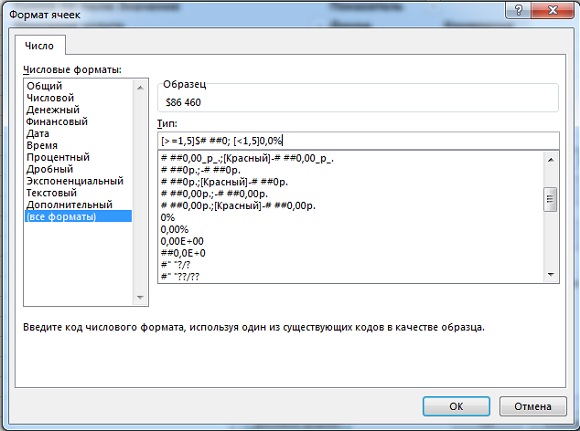
Figure: 21. Apply a custom number format where any numbers less than 1.5 are formatted as percentages

The result is shown in Fig. 22. As you can see, now each indicator is formatted correctly. Of course, the recipe in this tip is not universal. Rather, it indicates the direction in which to experiment.

Tip 13: Create a frequency distribution for the pivot table

If you have ever generated frequency distributions using Excel function Frequency, you probably know that this is a very difficult task. Moreover, after changing data ranges, everything has to start over. In this section, you will learn how to create simple frequency distributions using a simple pivot table. First, create a pivot table with the data in the row area. Pay attention to fig. 23, where the field is in the row area Volume sales.

Right click on any value in the Rows area and select the option from the context menu Group... In the dialog box Grouping (Fig. 24) determine the values \u200b\u200bof the parameters that determine the beginning, end and step of the frequency distribution. Click OK.

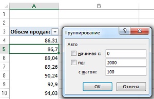
Figure: 24. In the dialog box Grouping adjust the frequency distribution parameters

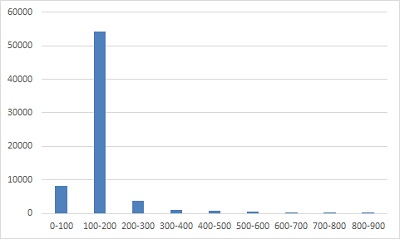
If you add a field to the pivot table Customer (Fig. 25), we get the frequency distribution of customer transactions relative to the size of orders (in dollars).

Figure: 25. Now you have at your disposal the distribution of customer transactions according to order sizes (in dollars)

The advantage of this technique is that the PivotTable report filter can be used to interactively filter data based on other columns, such as Region and Sales market... The user also has the ability to quickly adjust the frequency distribution intervals by right-clicking on any number in the row area and then selecting an option Group... For clarity of presentation, a pivot chart can be added (Fig. 26).

Tip 14. Using a pivot table to distribute a dataset across worksheet sheets

Analysts often have to create different PivotTable reports for each region, sales area, manager, etc. This task usually involves a lengthy process of copying the pivot table to a new sheet and then modifying the filter field to reflect the appropriate region and manager. This process is manual and repeated for each analysis. But in fact, you can outsource the creation of individual pivot tables to Excel. As a result of applying the parameter a separate pivot table is automatically created for each item in the filter fields area. To use this feature, simply create a pivot table that includes a filter field (Figure 27). Place your cursor anywhere in the pivot table and on the tab Analysis in the team group Pivot table click on the dropdown Options (fig. 28). Then click on the button Show Report Filter Pages.

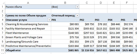
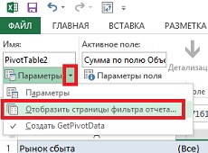
Figure: 28. Click the button Show Report Filter Pages

In the dialog box that appears (Figure 29), you can select a filter field for which separate pivot tables will be created. Select the appropriate filter field and click OK.

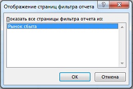
Figure: 29. Dialog box Displaying Report Filter Pages

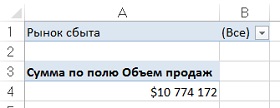
For each element of the filter field, a pivot table will be created, placed on a separate sheet (Fig. 30). Note that sheet tabs are named the same as items in the filter field. Note that the parameter Show filter pages can be applied to filter fields one by one.

Tip 15: Using a pivot table to distribute a dataset across individual workbooks

In tip 14, we used a special option to split summary tables by sales markets on different sheets of the workbook. If you need to split initial data for different markets in separate books, you can use a little VBA code. First, place the field you want to filter on in the filter fields area. Place the field Volume of sales into the range of values \u200b\u200b(Fig. 31). The suggested VBA code selects each FILTER item in turn and calls the function Show detailsby creating a new data sheet. This sheet is then saved in a new workbook

The code VBA.

Sub ExplodeTable ()

Dim PvtItem As PivotItem

Dim PvtTable As PivotTable

Dim strfield As PivotField

‘Change variables according to script

ConststrFieldName \u003d "Marketplace" ‘<—Изменение имени поля

Const strTriggerRange \u003d "A4" '<—Изменение диапазона триггера

'Change the name of the pivot table (if necessary)

SetPvtTable \u003d ActiveSheet.PivotTables ("PivotTable1") '<—Изменение названия сводной

‘Cycle through each element of the selected field

For Each PvtItem In PvtTable.PivotFields (strFieldName) .PivotItems

PvtTable.PivotFields (strFieldName) .CurrentPage \u003d PvtItem.Name

Range (strTriggerRange) .ShowDetail \u003d True

'Assigning a name to a temporary sheet

ActiveSheet.Name \u003d "TempSheet"

'Copying data to a new workbook and deleting a temporary sheet

ActiveSheet.Cells.Copy

ActiveSheet.Paste

Cells.EntireColumn.AutoFit

Application.DisplayAlerts \u003d False

ActiveWorkbook.SaveAs _

Filename: \u003d ThisWorkbook.Path & "\\" & PvtItem.Name & ".xlsx"

ActiveWorkbook.Close

Sheets ("Tempsheet") .Delete

Application.DisplayAlerts \u003d True

Enter this code into a new VBA module. Check the values \u200b\u200bof the following constants and variables and change them if necessary:

• Const strFieldName. The name of the field used to separate data. In other words, it is a field that fits in the filter / pages area of \u200b\u200bthe pivot table.
• Const strTriggerRange. A trigger cell that stores a single number from the data area of \u200b\u200bthe PivotTable. In our case, the trigger cell is A4 (see Fig. 31).

As a result of executing the VBA code, the data for each sales area will be saved in a separate workbook.

Note based on Jelen's book, Alexander. ... Chapter 14.

We recommend reading

Windows instructions

Cough after and during meals: reasons for what to do

Windows instructions

Useful properties and contraindications for the use of barberry

Android instructions

A wen appeared on the eyelid: causes, negative consequences and methods of treatment

Windows instructions

Total protein: what is it and its norm in a blood test

Android instructions

Uterine cancer: first signs and symptoms, early treatment

Windows instructions

Causes of coughing while eating