The difference is in excel. Calculating the difference in Microsoft Excel

Instructions

If you need to calculate the difference between two numbers using this spreadsheet editor, click the cell in which you want to see the result and enter an equal sign. If the contents of a cell start with this character, Excel assumes that there is some kind of mathematical operation or formula placed in it. After the equal sign, without a space, type the number to be reduced, put a minus and enter the number to be subtracted. Then press Enter, and the cell displays the difference between the two numbers entered.

Change the procedure described in the first step slightly if the numbers to be subtracted or subtracted should be taken from some other cell in the table. For example, so that cell B5 displays the number 55 reduced from cell D1, click B5, enter an equal sign, and click cell D1. After the equal sign, a link to the cell you specified will appear. You can also type its address manually, without using a mouse. Then enter the subtraction sign, the number 55 and press Enter - Excel will calculate and display the result.

To subtract the value of one cell from the value of another, use the same algorithm - enter an equal sign, type an address, or click the cell with the value to be decreased. Then put a minus, enter or click the cell with the value to be subtracted and press the Enter key.

If you want to create an entire column of cells containing the difference in numbers from other columns in each row of the table, start by creating one such cell in the first row. Do this according to the algorithm described in the previous step. Then move the cursor to the lower right corner of the cell with the subtraction formula and drag it down with the left mouse button to the last row of the table. Excel will change the links in the formulas for each row by itself when you release the left button.

Sooner or later, the user personal computer have to deal with software like Excel. These are designed spreadsheets that allow you to create various databases.

Instructions

To learn how to work with this program, you must first of all decide on the tasks that should be performed for you. Typically like software has flexible built-in functions that allow you to format and classify all information by different directions... There are many different courses on the Internet that allow you to see in real time how tables are built, information is integrated, data is sorted, and much more.

Typically, the first teaching begins with an introduction. You should be clear about where each graph is. At the moment there are several versions of this software, namely: Excel 2003, 2007 and 2010. Probably, many are accustomed to version 2003. Despite the fact that now updates are being created only for 2007 and 2010, Excel 2003 software does not stop popular.

Open the program on your computer. Go to the "Help" tab and read the items that interest you. In fact, such software is similar in function to Word. There are the same formatting commands, the menu items are very similar, the interface is also clear. To add a new table, click File - New. Next, enter the name of the document in which you will work.

Next, enter the information in the cells of the table. You can stretch each block, both in width and length. To add more cells, right-click on the table and select "Add Cells". In the "Service" tab, you can find additional operations that this software provides. Start by simply copying information into a table, and then try to display it in a table in different ways, sort it, try to present it in a more convenient form.

Related Videos

The Microsoft Office Excel spreadsheet editor has row numbering - these numbers can be seen to the left of the table itself. However, these numbers are used to indicate the coordinates of the cells and are not printed. In addition, the beginning of a user-created table does not always fit into the very first cell of a column. To eliminate such inconveniences, you have to add a separate column or row to the tables and fill it with numbers. You do not need to do this manually in Excel.

You will need

Microsoft Office Excel spreadsheet editor 2007 or 2010.

Instructions

If you need to number the data in an existing table, in the structure of which there is no column for this, you will have to add it. To do this, select the column in front of which the numbers should stand by clicking on its heading. Then right-click the selection and choose Paste from the context menu. If the numbers need to be placed horizontally, select the line and add an empty line through the context menu.

Enter the first and second numbers in starting cells column or row selected for numbering. Then select both of these cells.

Move the mouse pointer over the lower right corner of the selection - it should change from a raised plus to a black and flat plus. When this happens, press the left mouse button and drag the border of the selection to the very last cell of the numbering.

Release the mouse button, and Excel will fill in all the cells selected in this way with numbers.

The described method is convenient when you need to number a relatively small number of rows or columns, and for other cases it is better to use another version of this operation. Start by entering a number in the first cell of the created row or column, and then select it and expand the Fill drop-down list. On the "Home" tab in the spreadsheet editor menu, it is placed in the "Edit" command group. Select the Progression command from this list.

Specify the direction of the numbering by checking the box next to "by rows" or "by columns".

In the "Type" section, select the method of filling the cells with numbers. Regular numbering corresponds to the item "arithmetic", but here you can set and increase the numbers exponentially, as well as set the use of several options for calendar dates.

For regular numbering, leave the default (one) in the Step field, or enter the desired value if the numbers are to be incremented at a different rate.

In the "Limit value" field, specify the number of the last cell to be numbered. Then click OK, and Excel will fill the column or row with numbers according to the specified parameters.

Fix cell spreadsheetcreated in Excel, which is included in the Microsoft Office suite, means creating an absolute link to the selected cell... This action is standard for excel programs and is performed by regular means.

Instructions

Call the main system menu by clicking the "Start" button, and go to the "All Programs" item. Expand the Microsoft Office link and start Excel. Open the application workbook to be edited.

An absolute reference in table formulas is used to indicate a fixed cell address. Absolute references remain unchanged during move or copy operations. By default, when you create a new formula, a relative reference is used, which can change.

Highlight the link to be anchored in the formula bar and press the F4 function key. This action will cause a dollar sign ($) to appear in front of the selected link. Both the line number and the letter of the column will be fixed in the address of this link.

Press the F4 function key again to fix only the line number in the address of the selected cell. This action will cause the row to remain unchanged and the column to move as you drag formulas.

The next press of the F4 function key will change the cell address. Now the column will be fixed in it, and the row will move when moving or copying the selected cell.

Another way to create absolute cell references in Excel is to manually do the link pin operation. To do this, when entering a formula, you must print a dollar sign in front of the column letter and repeat the same action before the line number. This action will cause both of these parameters of the address of the selected cell to be fixed and will not change when you move or copy this cell.

Save your changes and exit Excel.

MS Excel has an extremely interesting feature that few people know about. So little that this function in Excel does not even provide contextual hints when typing, although, oddly enough, the help for the program has it and is described quite well. It is called DATED () or DATEDIF () and serves to automatically calculate the difference in days, months or years between two specified dates.

Doesn't sound good? In fact, sometimes the ability to quickly and accurately calculate how much time has passed since some event is very useful. How many months have passed since your birthday, how long have you been sitting in your pants at this place of work, or how many days have you been on a diet - are there any uses of this useful function? And most importantly, the calculation can be automated and every time you open an MS Excel workbook, you can receive accurate data for today! Sounds interesting, doesn't it?

The DATEDIF () function takes three arguments:

Start date - date from which the account is kept
Final date - to which the account is kept
unit of measurement - days, months, years.

It is written like this:

\u003d DATEDATE (start date; end date; unit)

Measurement units are written as:

"Y" - date difference in full years
"M" - date difference in full months
"D" - date difference in full days
"Yd" - the difference in dates in days from the beginning of the year, excluding years
"Md" - the difference in dates in days, excluding months and years
"Ym" - the difference in dates in full months excluding years

In other words, to calculate my total age in years at the current moment, I write the function as:

\u003d DATEDATE (07/14/1984; 03/22/2016; "y")

Note that the last argument is always enclosed in quotation marks.

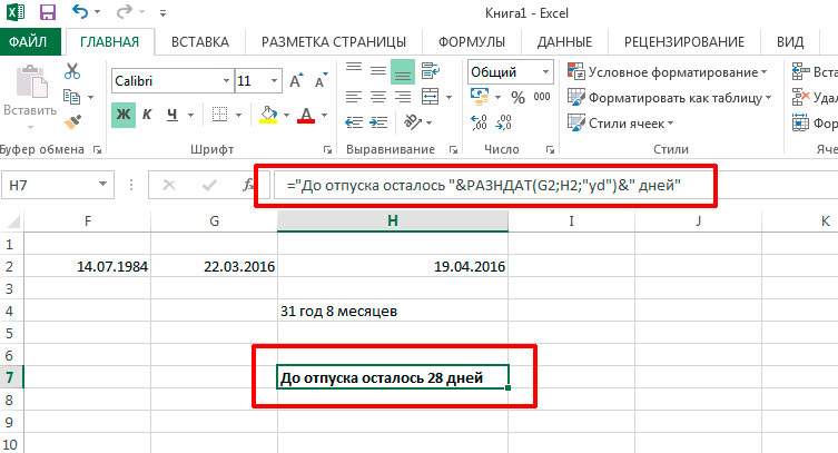
If I want to get the exact age, then I will write down a complicated formula:

\u003d DATEDIF (F2; G2; "y") & "year" & DATEDIF (F2; G2; "ym") & "months"

In which the RAZDAT () function is called twice at once, with different meanings, and the words "year" and "months" are simply docked to the result. That is, the real power of the function appears only when it is combined with other features of MS Excel.

Another interesting option - add to the function a counter moving daily relative to today's date. For example, if I decide to write a formula that calculates the number of days until my vacation in standard form, it will look something like this:

And everything would be correct if, opening this sheet a week later, I would see that the number of days before the vacation has decreased. However, I will see the same number as the original dates have not changed. Accordingly, I would have to change the current date, and then the DATEDAT () function would do everything right.

To avoid this annoying little thing, for the first argument (today's number), I will substitute not a reference to the value stored in the cell, but another function. This function is called TODAY () and its main and only task is to return today's date.

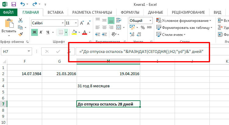
Once, and the problem is solved - from now on, whenever I open this MS Excel sheet, the RAZDAT () function will always show me the exact value calculated taking into account today's date.

Method 1: subtract numbers

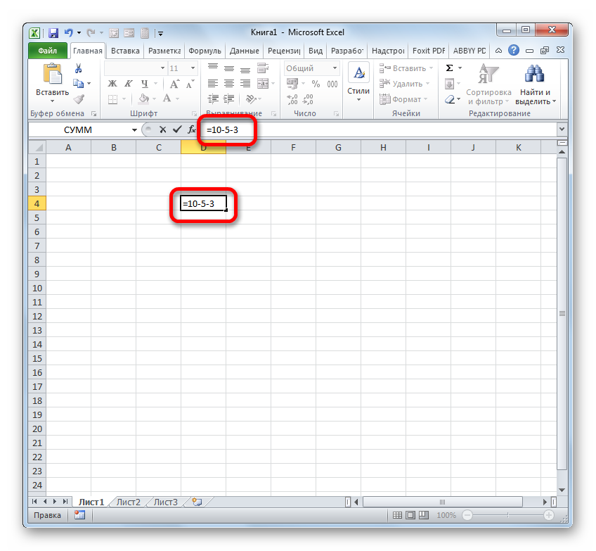
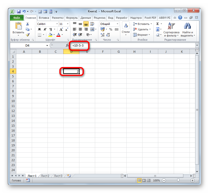
Let's go straight to the most commonly used variant of calculating the difference, namely subtracting numerical values. For these purposes, in Excel, you can apply the usual mathematical formula with a sign «-» .

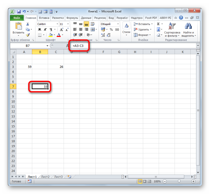
But much more often the process of subtraction in Excel is applied between numbers located in cells. At the same time, the algorithm of the mathematical operation itself practically does not change, only now, instead of specific numerical expressions, references to the cells where they are located are used. The result is displayed in a separate sheet element where the symbol «=» .

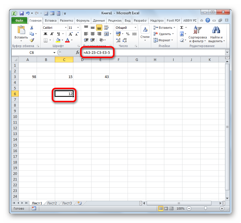
But in fact, in some cases, it is required to perform a subtraction, in which both the numerical values \u200b\u200bthemselves and the references to the cells where they are located will take part. Therefore, it is quite possible to meet an expression, for example, of the following form:

Method 2: currency format

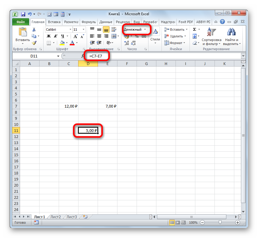
Calculating values \u200b\u200bin monetary format is practically no different from numeric ones. The same techniques are used, since, by and large, this format is one of the numeric options. The only difference is that at the end of the quantities taking part in the calculations, money symbol specific currency.

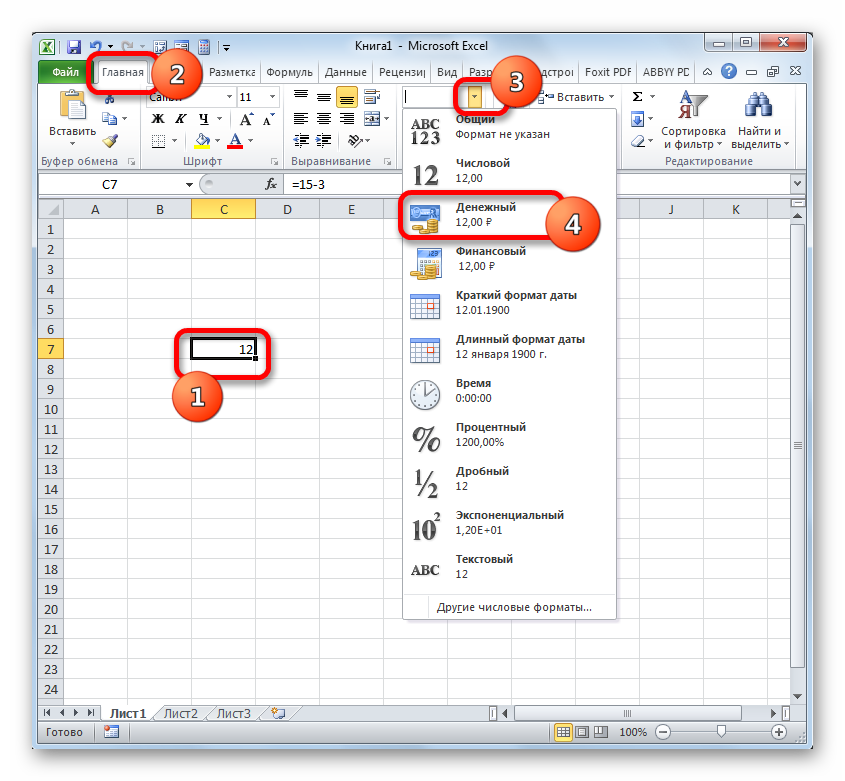
There is another option to format the resulting subtraction total for the monetary format. To do this, you need on the ribbon in the tab "The main" click on the triangle to the right of the display field of the current cell format in the tool group "Number"... From the list that opens, select the option "Monetary"... Numeric values \u200b\u200bwill be converted to monetary values. However, in this case there is no possibility to select the currency and the number of decimal places. The option that is set in the system by default, or configured through the formatting window, described above, will be applied.

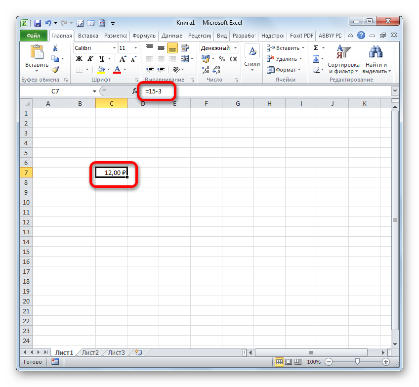
If you are calculating the difference between the values \u200b\u200bin cells that are already formatted for the currency format, then it is not even necessary to format the sheet element to display the result. It will be automatically formatted to the appropriate format after the formula is entered with links to elements containing the reduced and subtracted numbers, and the key is clicked. Enter.

Method 3: dates

But the calculation of the difference in dates has significant nuances that differ from the previous options.

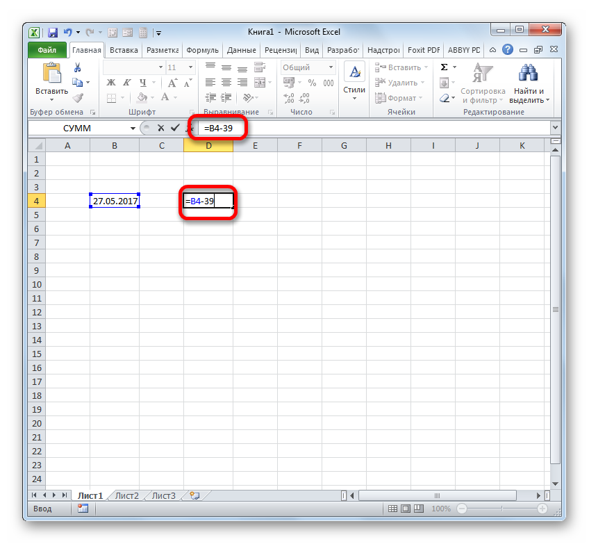
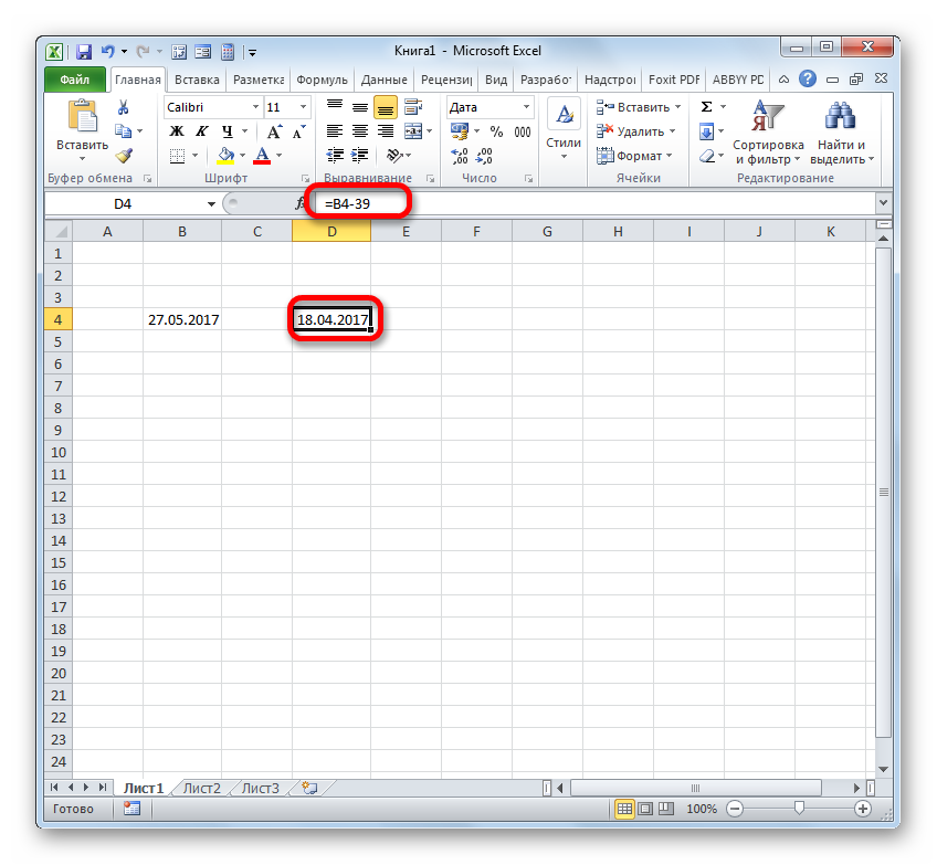
There is also the opposite situation, when it is required to subtract another from one date and determine the difference between them in days.

Also, the difference between dates can be calculated using the function DATED... It is good in that it allows you to configure, using an additional argument, in which units of measurement the difference will be displayed: months, days, etc. The disadvantage of this method is that working with functions is still more difficult than with ordinary formulas. In addition, the operator DATED not listed Function Wizards, and therefore will have to be entered manually using the following syntax:

DATEDATE (start_date; end_date; units)

"Start date" - an argument representing an early date or a link to it located in an element on the sheet.

"Final date" Is an argument in the form of a later date or a reference to it.

The most interesting argument "Unit"... With its help, you can choose an option for how the result will be displayed. It can be adjusted using the following values:

"D" - the result is displayed in days;
"M" - in full months;
"Y" - in full years;
"YD" - the difference in days (excluding years);
"MD" - the difference in days (excluding months and years);
"YM" - the difference in months.

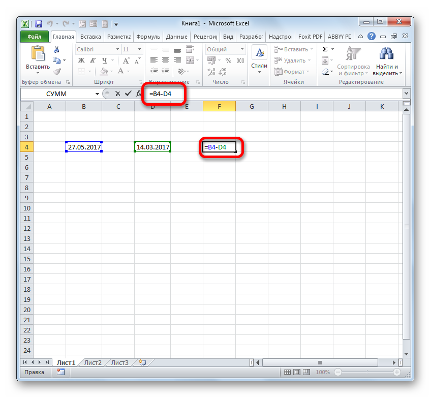
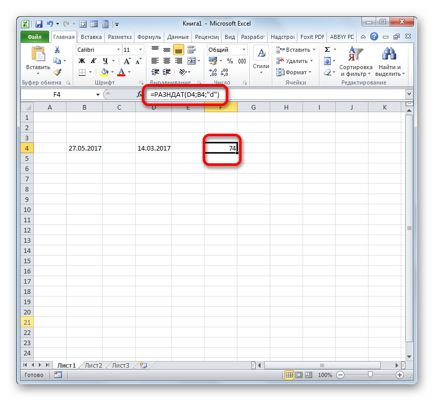
So, in our case, we need to calculate the difference in days between May 27 and March 14, 2017. These dates are located in cells with coordinates B4 and D4, respectively. We place the cursor on any empty sheet element where we want to see the calculation results, and write the following formula:

DATSDATE (D4; B4; "d")

Click on Enter and we get the final result of calculating the difference 74 ... Indeed, there are 74 days between these dates.

If you need to subtract the same dates, but without entering them into the cells of the sheet, then in this case we apply the following formula:

DATEDATE ("03/14/2017"; "05/27/2017"; "d")

Press the button again Enter... As you can see, the result is naturally the same, only obtained in a slightly different way.

Method 4: time

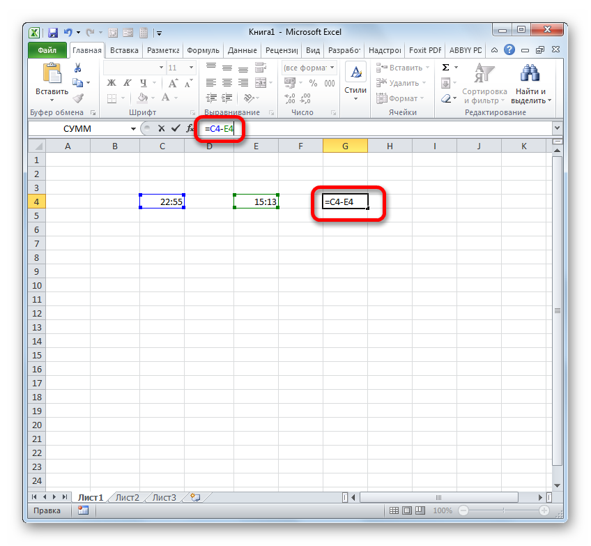
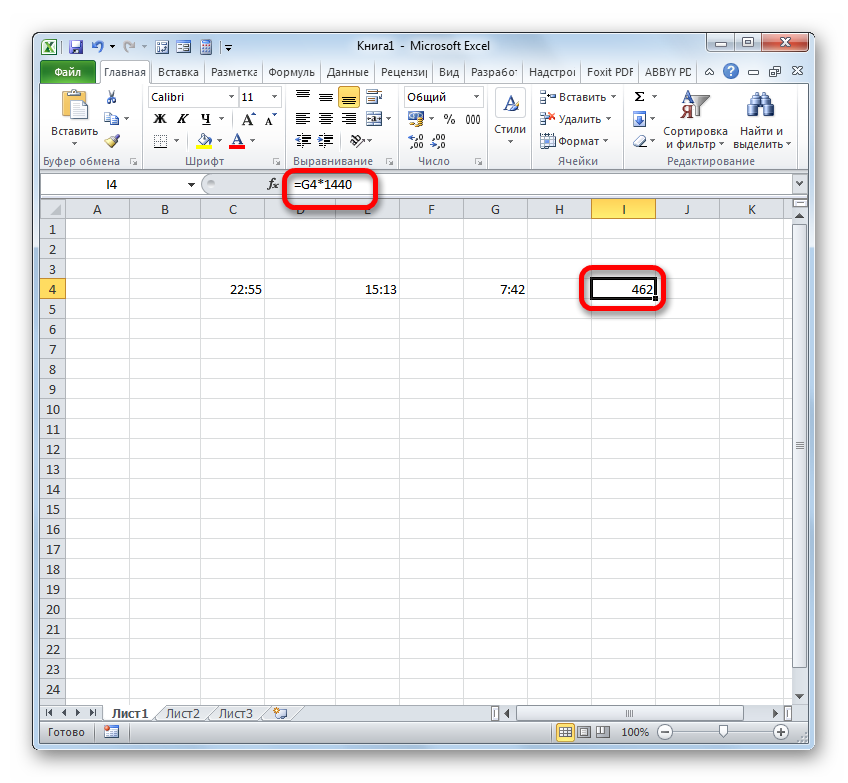
Now we come to the study of the algorithm for the subtraction of time in Excel. The basic principle is the same as for subtracting dates. It is necessary to subtract the earlier from the later time.

As you can see, the nuances of calculating the difference in Excel depend on what data format the user is working with. But nonetheless, general principle the approach to this mathematical action remains unchanged. Subtract another from one number. This can be achieved using mathematical formulas that are applied taking into account the special syntax of Excel, as well as using built-in functions.