How to write formulas in excel. Complete information about formulas in Excel
Microsoft program Excel Office has many convenient features that help you not to do long calculations before entering data into tables or charts. To calculate some values, for example, addition, subtraction, ratio, and others, you can use the originally specified formulas. You can add them yourself or choose from the list of existing ones. Learn to insert a formula step by step in this article.
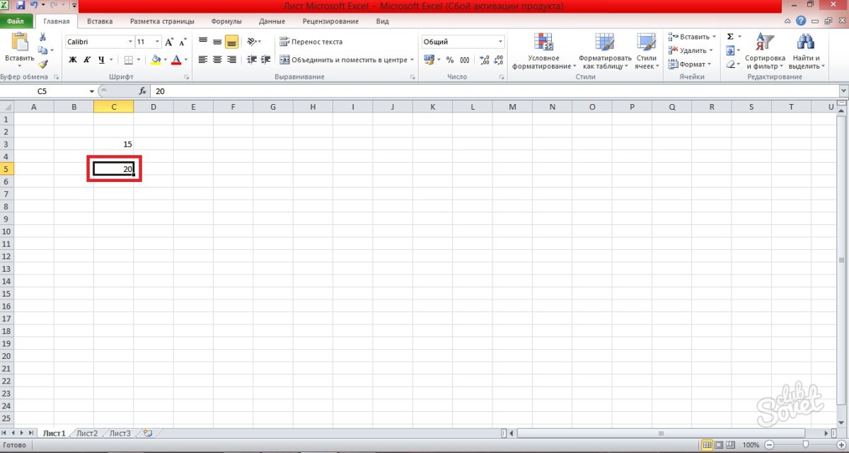
Open Excel. You will have a workspace in front of you, make sure the "Home" tab is open. In an empty line located between the program header and its work area, you will see a field for entering a formula, you will need it after entering the arguments, that is, the numbers that need to be calculated.


Now you know exactly how to create a formula in Excel and see their explanation in the function wizard.
If you haven't worked with Excel before, you will soon find out that this is not just a spreadsheet for entering numbers. Of course, in Excel, you can just count the amounts in rows and columns, but you can also calculate mortgage payments, solve mathematical and engineering problems, and find the most favorable options depending on the given variables.
In Excel, all this is done using formulas in cells. These formulas are used to perform calculations and other actions with the data on the worksheet. A formula always starts with an equal sign (\u003d), after which you can enter numbers, mathematical operators (such as the + and - signs for addition and subtraction), and built-in Excel functions that greatly expand the capabilities of formulas.
Below is an example of a formula that multiplies 2 by 3 and adds 5 to the result to get 11.
The following are examples of formulas that can be used on worksheets.
Parts of an Excel Formula
A formula can also contain one or more elements such as functions, links, operators and constants.
The order of actions in formulas
In some cases, the order of evaluation can affect the value returned by a formula, so it is important to understand the standard order of evaluation and know how to change it to get the results you want.
Using functions and nested functions in Excel formulas
Functions are predefined formulas that perform calculations on given values \u200b\u200b— arguments — in a specific order or pattern. Functions can be used to perform both simple and complex calculations. Everything excel functions can be seen on the Formulas tab.

Using links in Excel formulas
A link points to a cell or range of cells in a worksheet and tells Microsoft Excel, where the values \u200b\u200bor data required by the formula are located. Using links, you can use data in different parts of the worksheet in one formula, as well as use the value of one cell in multiple formulas. In addition, you can set links to cells in different sheets of one workbook or to cells from other books. References to cells in other books are called links or xrefs.
Using names in Excel formulas
To denote cells, cell ranges, formulas, constants, and excel spreadsheets you can create specific names. A name is a meaningful short designation that explains the purpose of a cell reference, constant, formula, or table, as it can be difficult to understand at a glance. The following are examples of names and how using them makes the formulas easier to understand.
Example 1
Example 2
Copy the sample data from the table below and paste it into cell A1 of the new excel worksheet... To display the results of formulas, select them and press F2, and then press Enter. In addition, you can adjust the width of the columns according to the data they contain.
Note: In the formulas in columns C and D, the specific name Sales is replaced with a reference to the range A9: A13, and the name Sales Information is replaced with the range A9: B13. If the book does not have these names, the formulas in D2: D3 will return the #NAME? Error.
|
Example type |
An example that does not use names |
An example using names |
Formula and result using names |
|
"\u003d SUM (A9: A13) |
"\u003d SUM (Sales) |
SUM (Sales) |
|
|
"\u003d TEXT (VLOOKUP (MAX (A9: 13), A9: B13,2, FALSE)," dd / mm / yyyy ") |
"\u003d TEXT (VLOOKUP (MAX (Sales), Sales Info, 2, FALSE)," dd.mm.yyyy ") |
TEXT (VLOOKUP (MAX (Sales), Sales Info, 2, FALSE), "dd.mm.yyyy") |
|
|
Date of sale |
|||
For more information, see the article Define and use names in formulas.
Using array formulas and array constants in Excel
An array formula can perform multiple calculations and then return a single value or group of values. An array formula processes multiple sets of values \u200b\u200bcalled array arguments. Each array argument must contain the same number of rows and columns. An array formula is created in the same way as other formulas, with the difference that you use CTRL + SHIFT + ENTER to enter the formula. Some built-in functions are array formulas and must be entered as arrays for correct results.
Array constants can be used instead of references if you do not need to enter each constant in a separate cell on the sheet.
Using an array formula to calculate one or more values
Note: When you enter an array formula, Excel automatically encloses it in curly braces (and). If you try to manually enter curly braces, Excel will display the formula as text.
Using array constants
In a regular formula, you can enter a reference to a cell with a value or to the value itself, also called a constant. Similarly, you can enter a reference to an array or an array of values \u200b\u200bcontained in cells (sometimes called an array constant) into an array formula. Array formulas accept constants in the same way as other formulas, however, the array constants must be entered in a specific format.
Array constants can contain numbers, text, Boolean values \u200b\u200bsuch as TRUE or FALSE, or error values \u200b\u200bsuch as # N / A. One array constant can contain values \u200b\u200bof various types, for example (1,3,4; TRUE, FALSE, TRUE). The numbers in array constants can be integer, decimal, or exponential. The text must be enclosed in double quotation marks, for example "Tuesday".
Make sure the following requirements are met when formatting array constants.
Constants are enclosed in curly braces ( { } ).
Columns are separated by commas ( , ). For example, to represent the values \u200b\u200b10, 20, 30, and 40, enter (10,20,30,40). This array constant is a 1-by-4 matrix and corresponds to a one row and four column reference.
Cell values \u200b\u200bfrom different lines are separated by semicolons ( ; ). For example, to represent the values \u200b\u200b10, 20, 30, 40, and 50, 60, 70, 80 in cells below each other, you could create a 2-by-4 array constant: (10,20,30,40; 50, 60,70,80).
Deleting a formula
Together with the formula, the results of its calculation are also deleted. However, you can delete the formula itself and leave the result of its calculation as the value in the cell.
Using a colon ( : ), the references to the first and last cells in the range are separated. For example: A1: A5.
Required arguments specified
A function can have required and optional arguments (the latter are indicated in the syntax with square brackets). All required arguments must be entered. Also, try not to enter too many arguments.
The formula contains no more than 64 levels of nesting of functions
Nesting levels cannot exceed 64.
Book and sheet names are enclosed in single quotes
If the names of the sheets or workbooks you reference cells or values \u200b\u200bcontain non-alphabetic characters, you must enclose them in single quotes ( " ).
The path to external books is specified
Numbers entered without formatting
You cannot use dollar signs when entering numbers in a formula, as they are used to indicate absolute references. For example, instead of the value $1000 need to enter 1000 .
Important: The calculated results of formulas and some Excel worksheet functions may differ slightly on x86 or x86-64 Windows computers and ARM-based Windows RT computers.
For a long time, all document flow has been carried out using computers and special applications. As a rule, almost all organizations, students, etc., for typing or performing calculations, use an office suite developed by Microsoft. In order to make high-quality tables in which values \u200b\u200bwill be automatically recalculated according to certain rules, you need to thoroughly study formulasExcel with examplesto simplify calculations.
Some cells in the table are calculated based on statistics that are entered in other cells. For example, if it is necessary to calculate the cost of several products sold in an invoice, the quantity is multiplied by the price and the result is the desired value. WITH spreadsheets it is much easier to do this, because by making one template and then changing some statistical values, recalculation is performed. For the result to be correct, you need to thoroughly know how to enter the formulas correctly, because otherwise, the calculation will be performed incorrectly. Let's consider several examples of simple formulas that are most often used, while they will clearly demonstrate the correctness of their compilation.
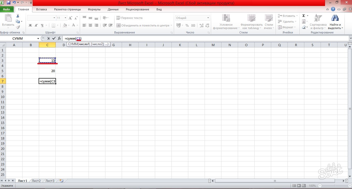
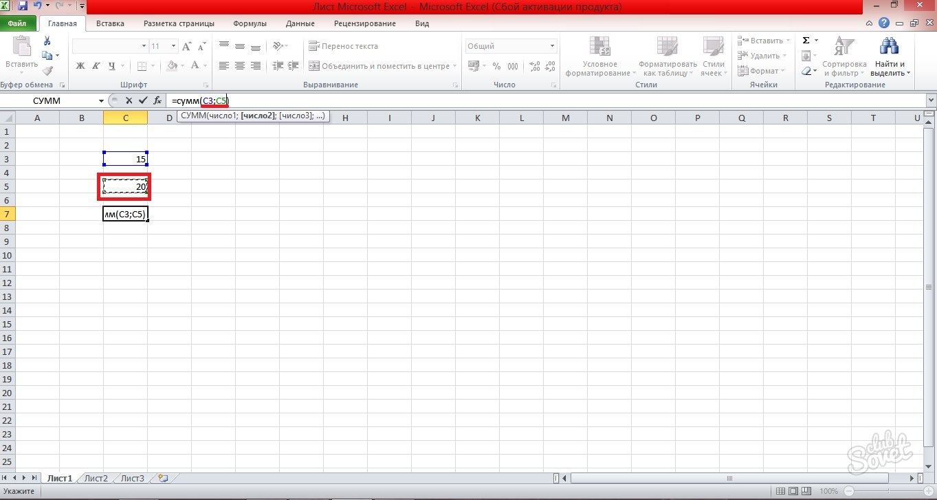
For the simplest example, let's calculate the sum of two values. To do this, in cell A1, write the number 5, and in B1, the number 3. For the sum to be calculated automatically, write the following combination of characters in cell C1, which will be the formula: \u003d SUM (A1; B1).
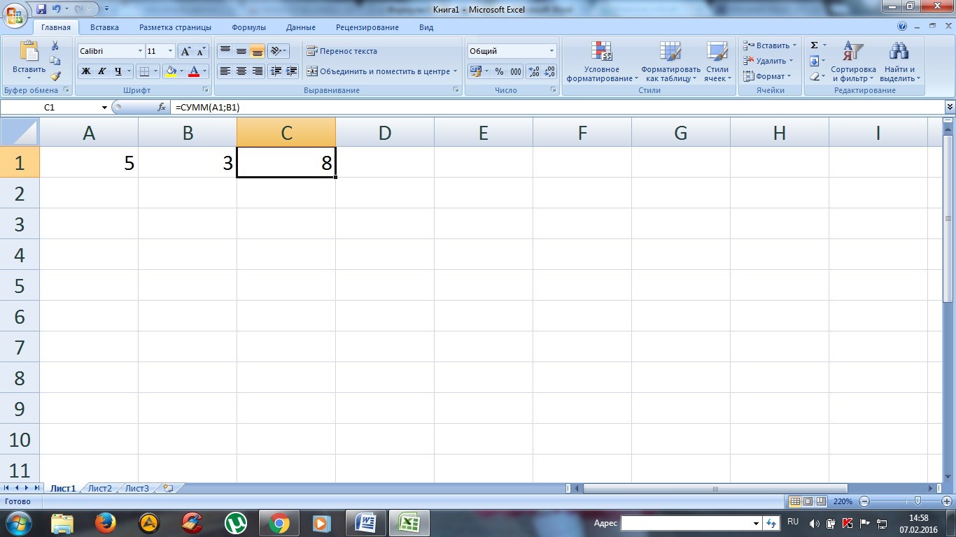
As a result, the calculated value will be displayed on the screen. Of course, it is not difficult to calculate such values, but if the number of terms is, for example, about 10, it is quite difficult to do it. When you change one of the entered values, the result will be automatically recalculated.
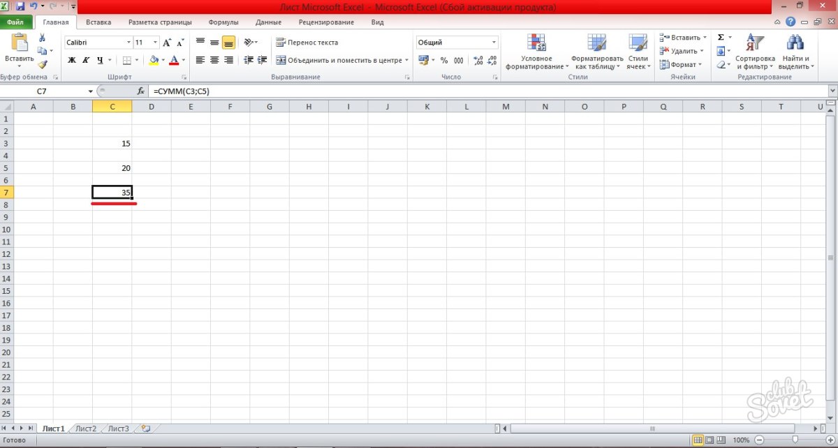
In order not to get confused where and what formula was spelled out, a line is displayed just above the table, in which the cell value is written (either statistical or a calculation formula).
In order to complicate the task, we introduce fractional numbers in cells A1 and B1, which are much more difficult to calculate. As a result, C1 will be recalculated and the correct value will be displayed.

In Excel, you can do not only addition, but also other arithmetic operations: subtraction, multiplication, division. The formula should always begin with the "\u003d" symbol and indicate the so-called coordinates of the cells (in this example, these are A1 and B1).
Create formulas yourself
In the above example, the formula \u003d SUM (A1; B1) allows you to add two values. The symbol "\u003d" is understood as the beginning of a formula, SUM is a service word that denotes the calculation of the sum, A1 and B1 are the coordinates of static values, which act as terms, and they must be separated by a semicolon ";".
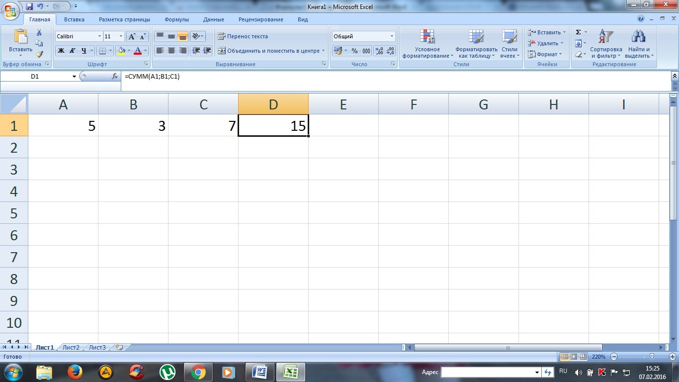
Consider an example of adding three cells A1, B1, C1. For this, an almost identical formula is written, but the third cell is additionally indicated in brackets. As a result, it is necessary to write the following combination \u003d SUM (A1; B1; C1) in cell D1 in order to perform the calculation.
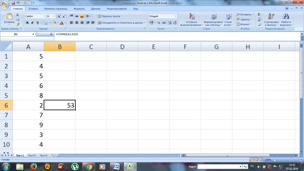
If there are quite a lot of terms that go in one row (column), for example 10, the formula can be simplified by specifying a range of coordinates. As a result, the formula will look like this: \u003d SUM (A1: A10). As a cell for displaying the desired result, select cell B6. As a result, we will get the result shown in the screenshot.
In order to multiply all the indicated values \u200b\u200bin the column, it is necessary to write PRODUCT in the formula instead of SUM.
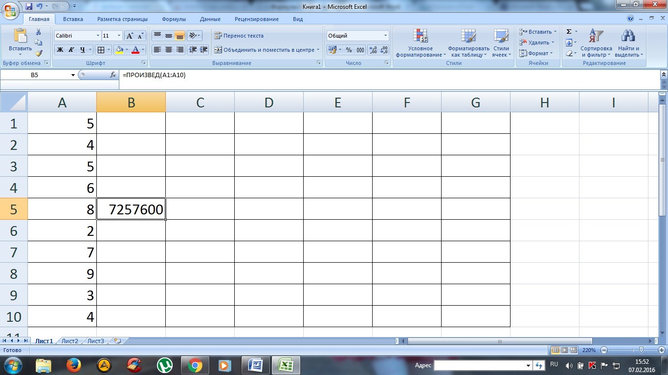
Note: if the user needs to perform addition or other arithmetic operation with several columns and rows, you can specify the coordinates diagonally opposite and an array of values \u200b\u200bwill be calculated (to calculate the product of the values \u200b\u200bof 10 rows in columns A, B, C, the formula will look like this : \u003d PRODUCT (A1: C10)).
Combined formulas
Spreadsheets are capable of performing not only simple arithmetic calculations, but also complex mathematical calculations.
For example, let's calculate the sum of the values \u200b\u200band multiply it by a factor of 1.4, if the value was less than 90 during the addition. If the result is greater than 90, then it should be multiplied by 1.5. In this case, the formula already contains several operators and looks much more complicated: \u003d IF (SUM (A1: C1)<90;СУММ(А1:С1)*1,4;СУММ(А1:С1)*1,5).

Two functions have already been used here instead of one: IF and SUM. The first command is a conditional statement that works like this:
- if the sum of three values \u200b\u200b(A1: C1) is greater than 90, multiplication is performed by 1.4, that is, by the first coefficient that is specified after the condition;
- if (A1: C1) is less than 90 (as in our given example), that is, the condition is not met, this value is multiplied by the second coefficient.
In our example, there are only two functions, but there can be much more, the program is practically unlimited in this.
Built-in functions in spreadsheets
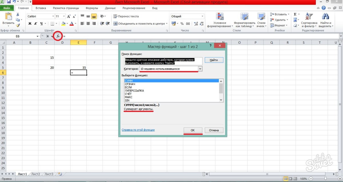
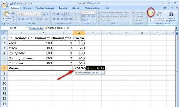
In order not to prescribe official words, you can use the special ability to install the function without dialing it. That is, to calculate the sum of values, you can use this feature and select a specific action for the specified range of values. There is a special button for this, shown in the screenshot.
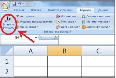
It is worth noting that there are quite a few functions there and many of them may not be needed, but some of them will be used regularly.

All functions are categorized to make it easier to find the one you want.
VLOOKUP function
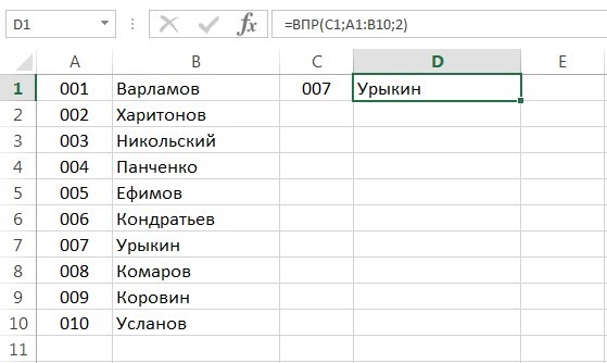
If the table consists of several hundred rows and it is not always possible to find the desired position, you can use the VLOOKUP function, which will search and return the result in the cell in which the formula is written.
For example, if we need to find the surname, which is assigned the serial number 007, we need to follow the steps that are clearly shown in the screenshot.
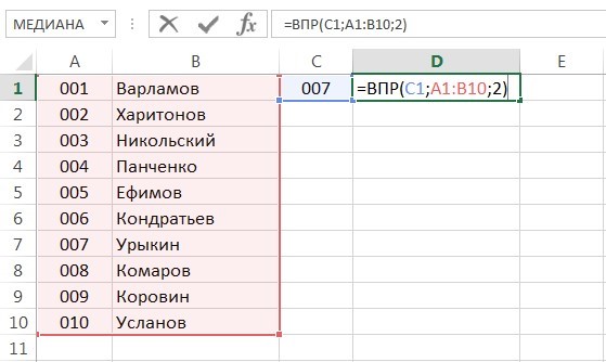
The value to search for is selected as the first argument. The range of values \u200b\u200bto search for is selected as the second argument. The number 2 indicates that the value from the second column should be displayed in this cell.
The result is the following result.
Rounding values
Excel can round up precisely to simplify calculations. There is a special function "ROUNDUP" for this. For example, if we need to round the number specified in cell A1, enter in the adjacent formula \u003d ROUNDUP (A1; 0), where the second argument shows to what order of decimal places it is tedious to round (if you specify zero, the total value will be an integer). The result is the following result.

As you can see from the screenshot, rounding up has occurred. In order to perform in a smaller, there is a function "ROUNDDOWN".
And although at first glance it seems that Excel spreadsheets are quite difficult to understand, you only need to work with them for a short time and feel that this statement is not entirely correct. In addition, the benefits of them are difficult to overestimate.
As you know, the Excel spreadsheet office editor was originally designed to perform mathematical, algebraic and other calculations, for which the input of special formulas is used. However, in the light of how to write a formula in Excel, it must be borne in mind that most of the input operations are fundamentally different from everything that is usually used in everyday life. That is, the formulas themselves have a slightly different form and use completely different operators that are used when writing standard calculations.
Let's consider the question of how to write a formula in Excel, using a few simple examples, without touching on complex operations, for understanding which you need to study the program deeply enough. But even prior knowledge will give any user an understanding of the basic principles of using formulas for different cases.
How to write a formula in Excel: basic concepts
So, the input of formula values \u200b\u200bin the program is somewhat different from the standard operations, the symbols used and the operators used. When solving the problem of how to write a formula in Excel, it is necessary to build on the basic concepts that are used in almost all computer systems.
The fact is that the machine does not understand the input of a combination like "2 x 2" or putting a common component outside the brackets ("2 + 2) 5"). For this, several types of symbols are provided, which are presented in the table below, not counting logical operators.
In this case, the priority of performing operations starts from the degree and ends with addition and subtraction. In addition, although Excel can be used like a regular calculator, as a rule, you must specify cell numbers or cell ranges for calculations. It goes without saying that the data format in any such cell must be set to the appropriate (at least numeric).
Sum and difference
How to write a sum or difference formula in Excel? So, let's start with the simplest, when you need to calculate the amount. In the line of formulas (moreover, for all operations), an equal sign is first entered, after which the desired formula is entered. In the case of a conventional calculator, you can specify for the installed cell "\u003d 2 + 2".
If the summation is performed for values \u200b\u200bentered directly in other cells (for example, A1 and A2), the formula becomes "\u003d A1 + A2". It is not uncommon to use parentheses to use additional operators. For the difference - the same thing, only with a minus instead of a plus.
When you need to specify the numbers of cells or their range, a special sum command can be used (in the Russian version "SUM", in English - SUM). When specifying several cells, it looks like this: "\u003d SUM (A1; A2)", for a range - "SUM (A1: A10)", provided that you need to calculate the sum of all numbers in cells from the first to the tenth. In principle, if you set the active cell, which is located immediately after the last one in the column with the initial values, you do not need to enter the formula, but simply click on the automatic summing button.
Multiplication, division and exponentiation
Now let's see how to write a multiplication or division formula in Excel. The order is the same as when entering a sum or difference, only the operators differ.

For the product the form is used "\u003d A1 * A2", for the quotient - "A1 / A2". By the way, these are exactly the same commands that can be found when using a standard Windows calculator.
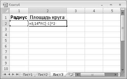
The symbol "^" is used for exponentiation. For the value in cell A1, which, for example, needs to be squared, the formula "\u003d A1 ^ 2" is applied.
Percentage calculations
With interest, if you do not touch on complex calculations, everything is also simple. How to write a formula with percentages in Excel?
It is enough to enter a formula of the form "\u003d A1 * 5%", after which you will get those very five percent of the value in the corresponding cell.
Using cell selection-based formula input
But all this related to manual assignment or the so-called direct input of formulas (direct or direct input). In fact, it is sometimes useful to use the mouse and the Ctrl key.

While holding down the mouse button, you can simply select the desired cells by first entering the required calculation in the formula bar. The cells will be added directly to the formula bar. But, depending on the type of formula, sometimes the parentheses will have to be entered manually.
Absolute, relative, and mixed cell types
It should be noted separately that the program can use several types of cells, not to mention the data they contain.
An absolute cell is unchanged and is denoted as $ A $ 1, relative is a reference to the usual location (A1), mixed - there is a combination of references to both absolute and relative cells ($ A1 or A $ 1). Typically, such formats are used when creating formulas when data are involved in different sheets of the book or even in different files. 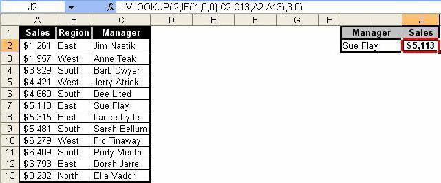
VLOOKUP formulas
Finally, let's see how to write a VLOOKUP formula in Excel. This technique allows you to insert data from one range into another. In this case, the method is somewhat similar to that used in solving the problem of how to write the "Condition" formula in Excel, which uses the symbols shown in the table above.
In general, such calculations are like a simple filter applied to columns, where you want to filter only exact values, not approximate values.
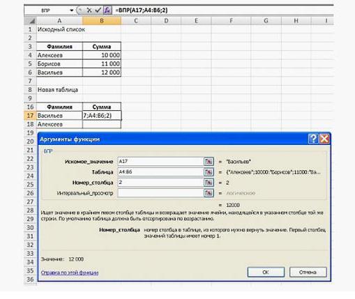
In this option, first through the "Function Wizard", the range of values \u200b\u200bof the original (first) table is used, the second range with fixing the contents (F4) is specified in the "Table" field, then the column number is indicated, and the value "FALSE" is set in the interval view field if indeed, when filtering, you really only need to get accurate, not approximate values. As a rule, such formulas are used more in warehouse or accounting, when it is not possible to install any specialized software products.
Conclusion
It remains to say that not all formulas that can be used in the Excel spreadsheet editor have been described here. This, so to speak, is just the basics. In fact, if you dig further into trigonometry or calculating logarithms, matrices, or even tensor equations, everything looks much more complicated. But in order to study all this, it is necessary to thoroughly study the manual for the editor itself. And this is not about the fact that in Excel, based on changing data, you can create even the simplest logic games. As an example, we can cite the same "snake", which initially had nothing to do with the spreadsheet editor, but was reproduced by enthusiasts in their field in Excel.
For the rest, it should be clearly understood that, having studied primitive formulas or actions with data, then it will be possible to easily master more complex calculations, say, with the creation of cross-references, the use of various kinds of scripts or VB scripts, etc. All this takes time, so if you want to study the program and all its possibilities to the maximum, you will have to sweat over the theoretical part.