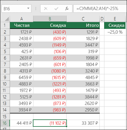
As in Excel to calculate the amount of the column. Addition of values \u200b\u200bin the column using the structure. Vertical aversion.

What is MS Excel? For many users, this is a program where there are tables that can be placed any information. But in fact, MS Excel has the greatest possibilities that most never think about, and can not imagine.

In this article, we consider one of the most important functions in MS Excel - the amount of cells. The developers were bored, creating this program. They worked out that the amount could be calculated not only single way, and a few. That is, you can choose yourself the easiest and most convenient way, and use it hereinafter.

Consider the input options in more detail, from the simplest, to more complex.

How to calculate the amount in MS Excel?

The search for the amount with the "+" sign is the easiest way and, accordingly, it is not necessary to search for anything here, since Plus is in Africa.

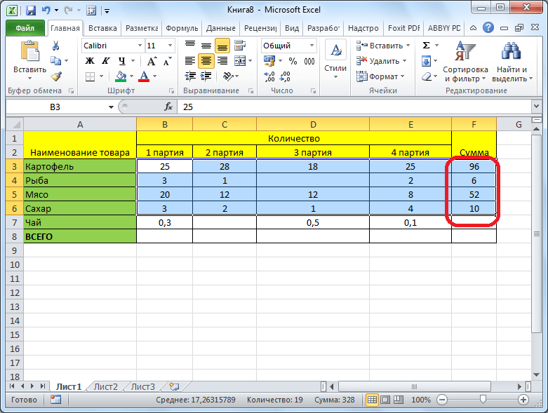
Suppose we are filled with three cells: A1, A2, A3 and we need to find their sum.

For this:

click on any free cell, in this case A4
print the sign "\u003d"
choose a cell a1
print sign "+"
choose a cell a2.
printed the "+" sign again
choose a cell a3
press the ENTER button

This option is good if you need to calculate a small number of values. And if their dozens?

How does MS Excel calculate the amount of the column (or lines)?

For this case, there are two ways: "Summage" button (autosumma) and the "\u003d amount ()" function.

Avosumn is a function, with which you can fold many cells at once in a few seconds.

Consider step by step:

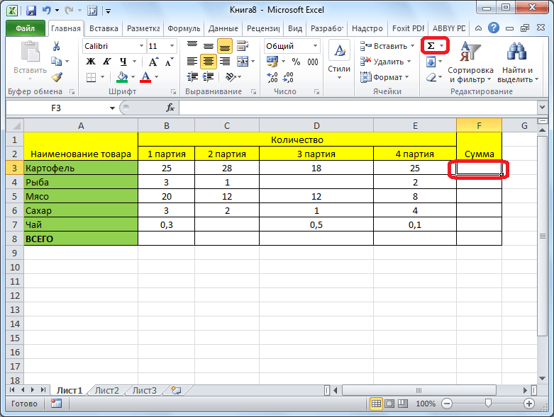
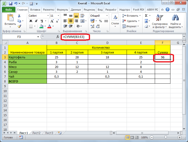
1. Select a free cell, in this case A5 (it is best to choose a cell under the numbers that we will add to the program to try to recognize the cells necessary to summarize)

2. Call the "Summage" function, for this serves special button On the toolbar

3. If Excel independently allocated the necessary cells, then you can do it manually by holding the left mouse button on the first cell and, without releasing the mouse button, stretch to the last, highlighting the entire range

4. Press the ENTER button to get the result

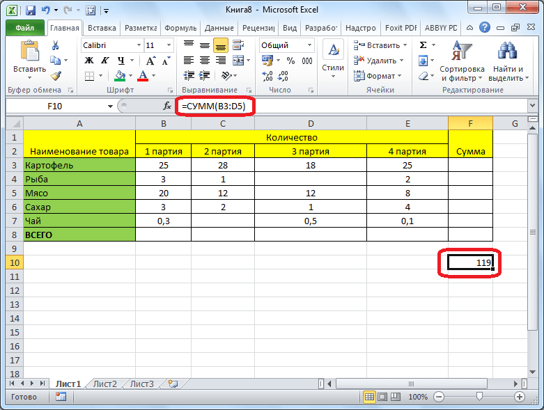
In turn, "\u003d amounts ()" (or SUM in the English version) is the simplest function that is not inferior to autosumma in which the range of cells are indicated in brackets, which we will summarize. The range can be prescribed both manually and highlight the mouse. There are two options to use this feature.

Option 1. Manual input.

1. Highlight a free cell

2. We introduce the formula "\u003d" to the line formula

3. Print the function of sums (A1: A4) (or SUM (A1: A4) in the English version), where A1: A4 - the range of the cells used

4. Press the ENTER button

By the way, if you use the second method in this embodiment, this formula can be edited as any other, and it is done right in the formula row. For example, you need to multiply the resulting value for two. To do this, in the formula string, we printe "* 2" and we get such a formula: \u003d sums (A1: A4) * 2.

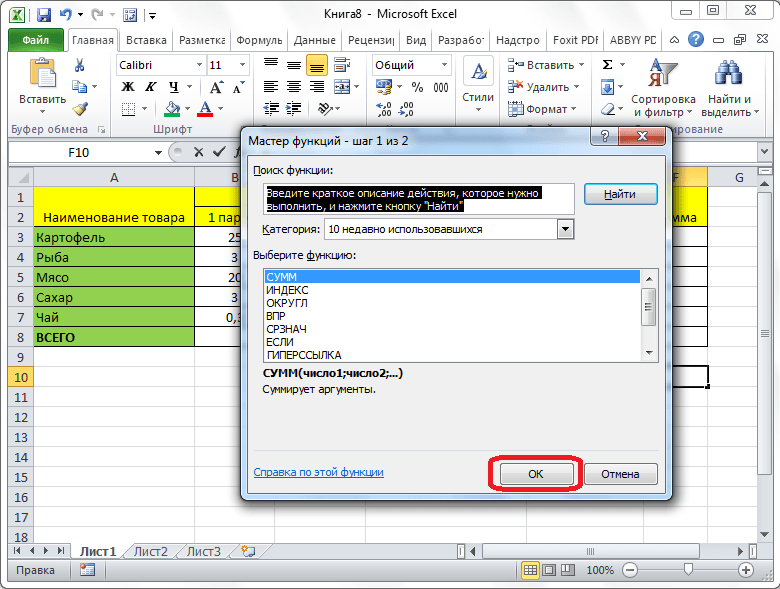
Option 2. Enter using a wizard of functions.

select a free cell in which summation will occur
click on the Master of Function Wizard: FX
in the dialog box, choose a category of the desired function, in this case "mathematical"
in the list of the list, select the "sums" function (or SUM) and click OK
select the required range of cells (B3: B20) and press the Enter key

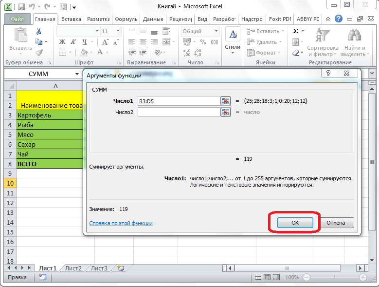
Again, the question arises: how to read the sum of different cells in MS Excel?

In this case, we can use both a simple sign "+" and the function "\u003d sums ()". Well, if in the first case everything is very simple and does not require explanations (RIS10), then with the second one must understand a little.

Suppose you need to fold individual cells from the table. What do we do for this:

1. As before choose a free cell and call the Master of Functions

2. Select the amount of the amounts

3. In brackets, alternately, separating the numbers from each other with a semicolon, select either the necessary cells, or the required ranges of cells

4. Press Enter key

Even more detailed description You can watch in the video: http://www.youtube.com/watch?v\u003dNK04P2JKGWK
However, with large amounts of information, it is possible that we will need to summarize not all values, but only those that correspond to certain conditions.

How to calculate the amount with the condition in MS Excel?

For this option, the "\u003d silent ()" function will be used. There are of course other functions, but this feature is more appropriate.

The general form of recording this feature is silent (range; Criterion; Range_Suming), where the "range" is a data range where the conditions for the condition, the "criterion" - is a specific condition that will be checked in this range, and the "media range" is The range from which the values \u200b\u200bcorrespond to the specified condition are selected.

Consider gradually on the example. Suppose we have a finished table and we need to determine the total value of all products of one name.

For this:

below finished table We repeat the string with the names of the columns and introduce every product name, but only without repetition
select the cell in which the summation will occur (D15) and call the Master of Functions
in the dialog box, we introduce the parameters of our function: Range - B2: B11 - Product Names, Criterion - B15 - Content Interest Interest, Range_Suming - F2: F11 - cost that will be summed.
click OK and get the result

Naturally, as in the previous cases, the formula can be prescribed manually.

More detailed description you can view in the video:

So we reviewed the basic functions for summation. Good luck to you when using MS Excel. Thanks for attention!

While working in the program Microsoft Excel. Often it is necessary to firm the amount in columns and rows of tables, as well as simply determine the amount of the range of cells. The program provides several tools to solve this issue. Let's figure out how to summarize cells in Excel.

The most famous and convenient tool to determine the amount of data in the cells in the Microsoft Excel program is Austosumma.

The program displays the formula into the cell.

In order to view the result, you need to click on the ENTER button on the keyboard.

You can do and a little differently. If we want to fold the cells of the entire row or column, but only a certain range, then we allocate this range. Then click on the already familiar button for the "Avosumn" button.

The result is immediately displayed.

The main disadvantage of counting using a self-seeming is that it allows you to calculate the serial number of the data in one line or in the column. But an array of data located in several columns and strings cannot be calculated in this way. Moreover, with it, it is impossible to count the sum of several cells distant from each other.

For example, we highlight the range of cells, and click on the "Avosumn" button.

But the screen is displayed not the sum of all these cells, but amounts for each column or lines separately.

Function "sums"

In order to view the amount of a whole array, or multiple data arrays in Microsoft Excel, there is a "sums" function.

We highlight the cell in which we want the amount to be displayed. Click on the "Insert function" button, located on the left of the formula string.

The Master of Function Wizard opens. In the list of functions we are looking for the "sums" function. We highlight it, and click on the "OK" button.

In the function of the arguments of the function, we introduce the coordinates of the cells whose amount is going to count. Of course, manually enter the coordinates are inconvenient, so I click on the button that is located to the right of the data entry field.

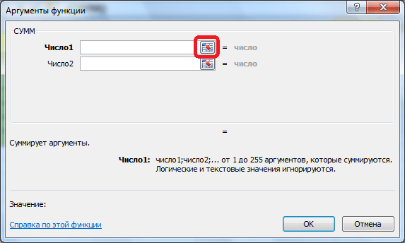
After that, the argument window is folded, and we can select those cells, or cells of the cells, the amount of the values \u200b\u200bof which we want to count. After the array is allocated, and its address appeared in a special field, press the button to the right of this field.

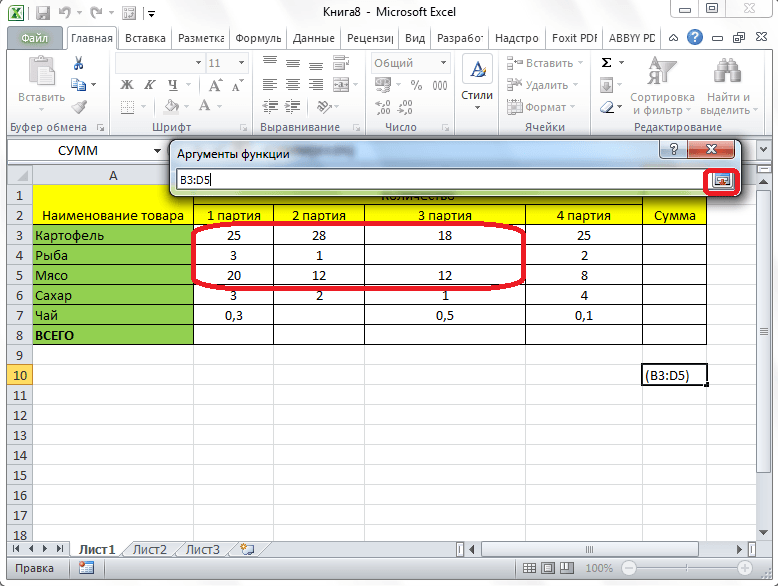
We come back in the function arguments window. If you need to add another array of data in a total amount, we repeat the same actions mentioned above, but only in the field with the "number 2" parameter. If necessary, similarly, you can enter the addresses of a practically unlimited amount of arrays. After all the function arguments are entered, press the "OK" button.

After that, in the cell in which we set out the output, the total amount of these cells is displayed.

Use of formula

The amount of data in the cells in the Microsoft Excel program can also be calculated using a simple formula of addition. To do this, we allocate the cell in which the amount should be, and put the sign "\u003d". After that, alternately click on each cell, from those whose amount of the values \u200b\u200byou need to calculate. After the cell's address is added to the formula string, enter the "+" sign from the keyboard, and so after entering the coordinates of each cell.

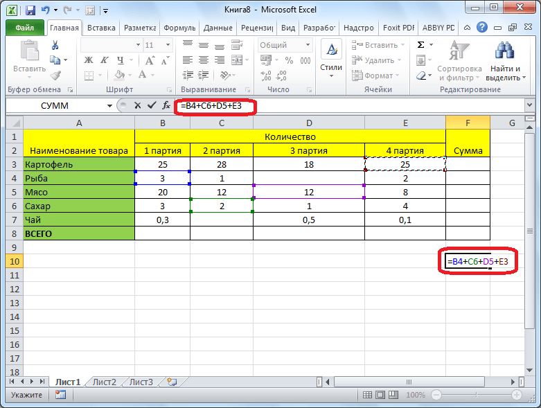
When the addresses of all cells are entered, we click the ENTER button on the keyboard. After that, the total amount of data entered in the specified cell is displayed.

The main disadvantage of this method is that the address of each cell has to be entered separately, and the range of cells cannot be allocated immediately.

View the amount in Microsoft Excel

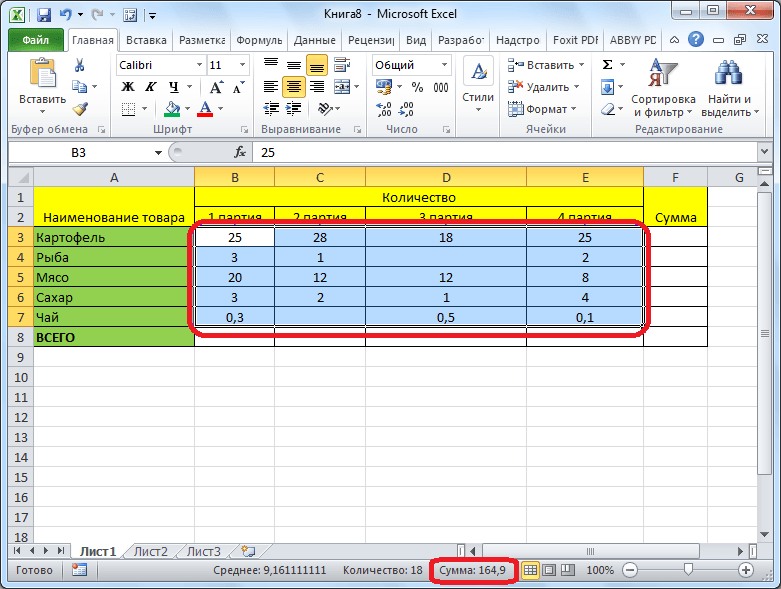
Also, the Microsoft Excel program has the opportunity to view the amount of selected cells without removing this amount in separate cell. The only condition is that all cells whose amount should be calculated should be nearby in a single array.

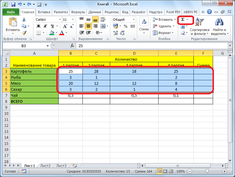
Simply select the range of cells, the amount of these data needs, and see the result in the status bar of the Microsoft Excel program.

As you can see, there are several ways to summarize data in the Microsoft Excel program. Each of these methods has its own level of complexity and flexibility. As a rule, the more simple the option, that is less flexible. For example, when determining the amount using a car mosmy, you can only operate with data built in a row. Therefore, in each particular situation, the user himself must decide which method is more suitable.

Advanced user friend package microsoft programs Office understands that Microsoft Excel is not only a large and convenient table, but also a modern supercalculator with a huge number of functions. In this small lesson, we will teach you how to calculate the amount in Excel.

How to calculate the amount in the cell in Excel

If you need to insert any numbers into the cell, then it is not necessary to calculate it in advance on the calculator. The main thing is to remember that any of its own action in the cell should be started from the mark \u003d. For example, you need to calculate in Exel the amount of 5 + 7. Inside any cell print: "\u003d 5 + 7" and press ENTER.

Excel - how to calculate the amount of the column

Click on a blank cell under the column.
By pressing the SHIFT key, press the up arrow. You allocate all cells in the column whose amount you need to count.
At the top on the standard panel with different icons, locate the sum icon (it looks like this: σ). Press it. Congratulations, you counted the amount of the column in Excele! The result appeared in the cell under the column.

If you work in excel program: Build graphs, make up tables, various reports, etc., then to calculate the amount of data you will not need to search for a calculator. The amount of numbers in Excel is calculated in a couple of clicks with the mouse, and it can be done in various ways.

The easiest - will allow calculate the amount of cells, Highlight them and look at the status bar. Here will be indicated "mean" for all the values \u200b\u200brecorded in the selected cells, the "number" of the selected cells and the "sum of" values. Also, you can also empty cells and cells with text, only numbers are summed up.

If your table has a string "Results" - this method is not suitable. Of course, you can enter the number there, but if the data for the table changes, you need to not forget to change and value in the "Results" cell. This is not entirely convenient, and other methods can be used in Excel, which will automatically recalculate the amount in the column.

Calculate the sum in the column You can use the Autosumn button. To do this, highlight the last cell of the column, under the values. Then go to the Formulas tab and click Autosumn. Excel will automatically highlight the upper cells, to the first empty. Press "ENTER" to calculate the amount.

You can first select the cells in the column, considering and empty, and with the text - they will simply not be taken into account when calculating, and then click "Avosumn". The result will appear in the first empty cell of the selected column.

The most convenient way to calculate the amount in Excel is using the function of sums. Put "\u003d" in the cell, then type "sums", open the bracket "(" and highlight the desired range of cells. Set ")" and press "ENTER".

You can also register the function directly in the formula row.

If the argument for the amounts specify the range of cells in which cells with text or empty - the function will return the correct result. Since only cells with numbers will be taken into account for calculation.

Folding values. You can fold individual values, cell ranges, cell references or data of all these three species.

\u003d Sums (A2: A10)

\u003d Sums (A2: A10; C2: C10)

This video is part training course Addition of numbers in Excel 2013.

Syntax

Sums (number1; [number2]; ...)

Fast summation in the status bar

If you need to quickly get the amount of the range of cells, you just need to highlight the range and look at the lower right corner of the Excel window.

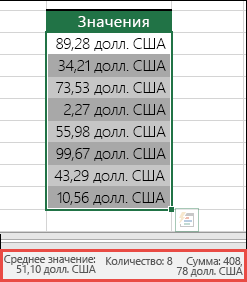
Status bar

Information in the status bar depends on the current dedicated fragment, whether it is one cell or several. If you right-click the status bar, a pop-up dialog box appears with all available parameters. If you select any of them, the corresponding values \u200b\u200bfor the selected range will appear in the status bar. For more information about the status bar.

Using Masters Aviamoving

The formula of sums is easiest to add to the sheet using the Avia Master. Select a blank cell directly above or under the range that you want to summarize, and then open the "Home" or "Formula" tab on the tape and click Avosumn\u003e Amount. Master of Aviation Automatically determines the range for summation and creates a formula. It can work horizontally if you choose a cell on the right or left of the summed range, but this will be considered in the next section.

Rapid addition of adjacent ranges using the Mastera of Aviation

In the Autosumn dialog box, you can also select other standard functions, for example:

Vertical aversion

Master of Aviation Automatically Determines Cells B2: B5 as a range for summation. You only need to press the Enter key to confirm. If you need to add or eliminate multiple cells while holding down the SHIFT key, press the appropriate arrow key until you select the desired range, and then press the Enter key.

Intellisense tip for function. Floating Tag amounts (number1; [Number2]; ...) Under the function is an IntelliSense tip. If you click the sums or name of another function, it will take the type of blue hyperlink, which will lead you to the help section for this function. If you click the individual elements of the function, the corresponding fragments will be highlighted in the formula. In this case, only cells B2: B5 will be allocated, since in this formula there is only one numerical link. IntelliSense tag appears for any function.

Horizontal aversion

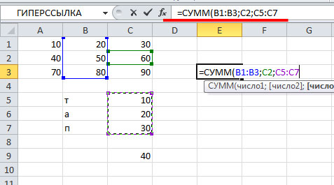
Using Functions for Continuous Cells

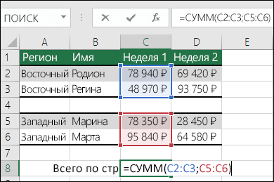
The autosumum wizard usually works only with adjacent ranges, so if your range for summation contains empty strings or columns, Excel will stop on the first pass. In this case, you need to use the function of the selection amounts in which you sequentially add separate ranges. In this example, if you have data in the B4 cell, Excel will create a formula \u003d Sums (C2: C6) because it recognizes the adjacent range.

To quickly select multiple non-magic bands, press Ctrl + click left mouse button. First enter "\u003d sums (", then select different ranges, and Excel will automatically add a point in the separator between them. Upon completion, press Enter.

Council. Quickly add a function of the amount in the cell using the keys Alt + \u003d.. After that, you will only have to select the ranges.

Note.You may notice that Excel highlights the color of different ranges of these functions and the corresponding fragments in the formula: C2 cells are highlighted in one color, and the C5 cells are different. Excel does it for all functions, if only the range on which the link indicates is not on another sheet or in another book. For more efficient use of special features, you can create named ranges, such as "Week 1", "Week 2", etc., and then refer to them in the formula:

\u003d Sums (week1; week 2)

Adding, subtraction, multiplication and division in Excel

In Excel, you can easily perform mathematical operations - both individually and in combination with excel features, for example amounts. The table below lists the operators that may be useful to you, as well as related functions. Operators can be entered both using a digital row on the keyboard and using a numeric keypad if you have it. For example, using the SHIFT + 8 keys, you can enter an asterisk sign (*) to multiply.

For more information, see Using Microsoft Excel as a calculator.

Other examples