As expected, what could be solved in MS Excel can be implemented in Google Sheets. But numerous attempts to solve problems with the help of your favorite search engine led only to new questions and almost zero answers.
Therefore, it was decided to make life easier for others and to glorify themselves.

Briefly about the main

In order for Excel or spreadsheet (Google spreadsheet) to understand that what is written is a formula, you must put the "\u003d" sign in the formula bar (Figure 1).

• alphanumeric (LETTER \u003d COLUMN; NUMBER \u003d LINE) eg "A1".
• in the R1C1 style, in the R1C1 system both rows and columns are designated by numbers.

The address of cell "B3" in such a system will look like R3C2 (R \u003d row \u003d row, C \u003d column \u003d column). For scripts, for example, both styles are used.
Where we write "\u003d formula", for example, \u003d SUM (A1: A10) and our value will be displayed.
The general operating principle of RC formulas is shown in Figure 2.

Picture 2
As you can see from Figure 3, the cell values \u200b\u200bare relative to the cell in which the formula with an equal sign will be written. To preserve the aesthetic appearance of the formulas, they contain symbols that can be omitted: RC \u003d RC.

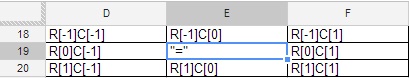
Figure 3
The difference between Figure 2 and Figure 3 is that Figure 3 is a generic formulation that is not tied to rows and columns (look at the values \u200b\u200bof rows and columns), which cannot be said about Figure 2. But the RC style in spreadsheet is mainly used for writing javascript scripts.

Link types (addressing types)

To refer to cells, links are used, which are of 3 types:

• Relative links (example, A1);
• Absolute links (example, $ A $ 1);
• Mixed links (example, $ A1 or A $ 1, they are half relative, half absolute).

The $ sign here indicates the type of link. You can see the differences between the different types of links by dragging on the autocomplete handle of the active cell or a range of cells that contain a formula with links.

Relative links

A relative link "remembers" at what distance (in rows and columns) you clicked RELATIVE to the position of the cell where you put "\u003d" (offset in rows and columns). Then pull down on the autocomplete handle, and this formula will be copied to all the cells we stretched through.

Absolute links

As mentioned above, if you drag a formula containing relative links on the autocomplete marker, the Table will recalculate their addresses. If the formula contains absolute links, their address will remain unchanged. Simply put - an absolute reference always points to the same cell.
To make a relative reference absolute, just put the "$" sign in front of the column letter and the row address, for example $ A $ 1. More quick way - select the relative link and press the "F4" key once, while the spreadsheet will put the "$" sign itself. If you press "F4" a second time, the link will become mixed type A $ 1, if the third time - $ A1, if the fourth time - the link will again become relative. And so in a circle.

Mixed links

Mixed links are half absolute and half relative. The dollar sign in them appears either before the letter of the column or before the line number. This is the most difficult link type to understand. For example, the cell contains the formula "\u003d A $ 1". Reference A $ 1 is relative in column A and absolute in row 1. If we drag this formula down or up on the autocomplete marker, the links in all copied formulas will point to cell A1, that is, they will behave as absolute. However, if we drag to the right or to the left, the links behave as relative, that is, the spreadsheet will begin to recalculate its address. Thus, formulas generated by autocomplete will use the same row number ($ 1), but the literal column value (A, B, C ...) will change.

Let's look at an example of summing cells with multiplication by a certain coefficient.

This example assumes the presence of a coefficient value in each calculated cell (cells D8, D9, D10 ... E8, F8 ...). (Figure 4).
The red arrows show the direction of stretching with the filling handle of the formula, which is in cell C2. In the formula, notice the change in cell D8. When stretching down, only the number that symbolizes the string changes. Stretching to the right only changes the column.

Figure 4
Let's simplify the example by using the $ sign (Figure 5).

Figure 5
But it is not always necessary to freeze all columns and rows, sometimes only row or only column freezing is used (Figure 6)

Figure 6
You can read about all the formulas on the official website support.google.com
Important: The data that needs to be processed in the formulas should not be in different documents, this can only be done using scripts.

Formula errors

If you misspell the formula, you will be notified by a comment about a syntax error in the formula (Figure 7).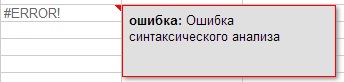

Figure 7
Although errors can be not only syntactic, but also, for example, mathematical, such as division by 0 (Figure 7) and others (Figure 7.1, 7.2, 7.3). To see a note showing which error occurred, hover over the red triangle in the upper right corner of the error.

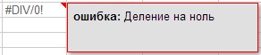
Figure 7.1

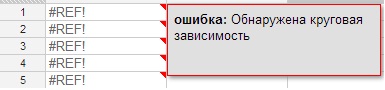
Figure 7.2

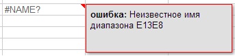
Figure 7.3
For the convenience of the table, all cells with formulas will be colored purple.
In order to see the formulas "live" you need to press the hot key Ctrl + or select View (View)\u003e All formulas from the top menu. (Figure 8).

Figure 8

How formulas are written

There are differences in the wording of formulas in the reference book and in the formulas that are used to work at the moment. They consist in the fact that instead of the "comma", which was used earlier in many formulas, the "semicolon" is already used (the changes took place more than half a year ago).
In order to see what the formula refers to on this page (Figure 9), you need to click in the formula bar to the right of the Fx label (Fx is located under the main menu, on the left).

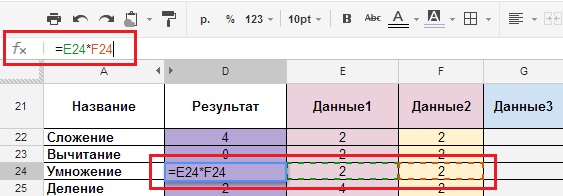
Figure 9
IMPORTANT: For the formulas to function correctly, they must be written in LATIN letters. Russian (Cyrillic) “A” or “C” and Latin “A” or “C” for the formula are 2 different letters.

Formulas

Arithmetic formulas.

Of course, no one will describe the eternal operations of addition, subtraction, etc., but they will help to understand the very basics. A few examples will show you how they work in this environment. All the formulas are given in the document, the link to which is given at the end of the article, but we will just stop at the screenshots.

Addition, subtraction, multiplication, division.

• Description: Formulas for addition, subtraction, multiplication and division.
• Formula type: “Cell_1 + Cell_2”, “Cell_1-Cell_2”, “Cell_1 * Cell_2”, “Cell_1 / Cell_2”
• The formula itself: \u003d E22 + F22, \u003d E23-F23, \u003d E24 * F24, \u003d E25 / F25.

We have the initial data in the range E22: H25 and the result in column D. Figure 10 shows the header for all the data that will be used.

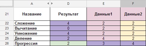
Figure 10

Progression.

• Description: the formula for increasing all subsequent cells by one (numbering of rows and columns).
• Formula type: \u003d Previous cell + 1.
• The formula itself: \u003d D26 + 1

Recall that if you want to use a range, it will sum all cells in a row, and if you need to sum cells in a certain order, then you need to specify them with “;” in the right order. We have the initial data for the progression in cell D26, and the result in cells E26: H26 (Figure 11) It is used to number rows and columns.

Figure 11

Rounding.

• Description: A formula for rounding a number in a cell.
• Formula type: \u003d ROUND (cell with a number); counter (how many digits must be rounded after the decimal point).
• The formula itself: \u003d ROUND (E28; 2).

We have the initial data in cell E28, and the result in cell D28 (Figure 12)

Figure 12
“ROUND” is rounded off by mathematical laws, if after the decimal point there is a digit 5 \u200b\u200bor more, then the whole part is increased by one, if 4 or less, then it remains unchanged, you can also round off using the FORMAT menu -\u003e Numbers -\u003e "1000,12" 2 decimal places (Figure 13 ). If you need more characters, then you need to click FORMAT -\u003e Numbers -\u003e Personalized decimal -\u003e And specify the number of characters.

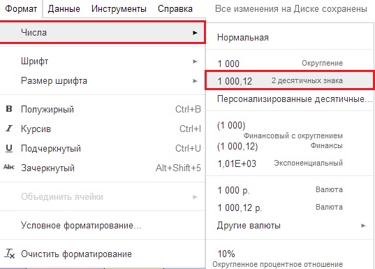
Figure 13

Amount if cells are not sequential.

Probably the most familiar feature

• Description: the sum of numbers that are in different cells.
• Formula type: \u003d SUM (number_1; number_2;… number_30).
• The formula itself: "\u003d SUM (E30; H30)" write through ";" if different cells.

We have the initial data in cells E30 and H30, and the result in cell D30

(Figure 14).
Amount if cells are sequential.

• Description: summation of numbers that follow one another (sequentially).
• Formula type: \u003d SUM (number_1: number_N).
• The formula itself: \u003d SUM (E31: H31) "write through": "if it is a continuous range.
• We have the initial data in the range of cells E31: H31, and the result in cell D31 (Figure 15).

Figure 15

Average.

• Description: the range of numbers is summed and divided by the number of cells in the range.
• Formula type: \u003d AVERAGE (cell with number or number_1; cell with number or number_2;… cell with number or number_30).
• The formula itself: \u003d AVERAGE (E32: H32)

We have the initial data in the range of cells E32: H32, and the result in cell D32 (Figure 16).

Figure 16
Of course, there are others, but we go further.

Text formulas.

Of the great number of textual formulas with which you can do anything you want with text, the most popular, in my opinion, is the formula for "gluing" text values. There are several options for its implementation:

Glueing text values \u200b\u200b(formula).

• Description: "gluing" text values \u200b\u200b(option A).
• Formula type: \u003d CONCATENATE (cell with number / text or text_1; cell with number / text or text_2;…, cell with number / text or text_30).
• The formula itself: \u003d CONCATENATE (E36; F36; G36; H36).

We have the initial data in the range of cells E36: \u200b\u200bH36, and the result in cell D36 (Figure 17).
Using Google Docs, they often conduct employee surveys or compose opinion polls through Google Forms (these are special forms that can be created through the Insert-\u003e Form menu. After filling out the form, the data is presented in a table. And then, they use various formulas to work with the data, for example , for gluing the full name).

Figure 17

Bonding numeric values.

• Description: “gluing” text values \u200b\u200bby hand, without using special functions (option B - manual writing of a formula, the complexity of the formula is any.).
• Formula type: \u003d cell with number / text 1 & "" & cell with number / text 2 & "" & cell with number / text 3 & "" & cell with number / text 4 ("" - space, & sign means gluing, all text values \u200b\u200bare written in quotation marks “”).
• The formula itself: \u003d E37 & "" & F37 & "" & G37 & "" & H37.

We have the initial data in the range of cells E37: H37, and the result in cell D36 (Figure 18 - glued numbers).

Figure 18

Bonding numeric and text values.

• Description: "gluing" text values \u200b\u200bby hand, without using special functions (variant C - mixed type, the complexity of the formula is any).
• Formula type: \u003d "text_1" & cell_1 & "text_2" & cell_2 & "text_3" & cell_3
• Important: all text that will be written in “” will be unchanged for the formula.
• The formula itself: \u003d "1 more" & E38 & "use" & F38 & "like US" & G38.

We have the initial data “1 more”, “use”, “like US” and in the range of cells E38: G38, therefore it is advisable to use this kind of formula, and the result is in cell D36 (Figure 19).
Glue text and numeric values \u200b\u200btogether.

Figure 19

LOGICAL AND OTHER

Transfer of data from any sheets of the same file.

We have come to the most interesting, in my opinion, functions: LOGICAL AND OTHER.
One of the most useful formulas:

• Description: transfer of data from any sheets of the same file (for Excel, you can transfer both from a sheet of one workbook to another sheet of the same workbook, or from a sheet of one workbook to a sheet of another workbook).
• Formula type: \u003d "Sheet_Name"! cell_1
• The formula itself: \u003d Data! A15 (Data is a sheet, A15 is a cell on that sheet).

We have the initial data on the Data sheet, cell A15 (Figure 20), and the result on the Formula sheet in cell D41 (Figure 20.1).

Figure 20

Figure 20.1

An array of formulas.

Most spreadsheet programs contain two types of array formulas: "multi-cell" and "single-cell".
Google Sheets divides these types into two functions: CONTINUE and ARRAYFORMULA.
Multi-cell array formulas allow a formula to return multiple values. You can use them without even knowing it, simply by entering a formula that returns multiple values.
One-cell array formulas let you write formulas using array input rather than output. When enclosing a formula in the \u003d ARRAYFORMULA function, you can pass arrays or ranges to functions and operators that typically only use non-array arguments. These functions and operators will be applied, one for each entry in the array, and will return a new array with all the output.
If you want to investigate in more detail, you should visit support.google.
In simple terms, to work with formulas that return arrays of data, in order to avoid syntax errors, you must enclose them in an array of formulas.

Summing cells with an IF condition.

In order to operate with logical formulas, which usually contain large arrays of data, they are placed in the array of formulas ARRAYFORMULA (formula).

• Description: Sum cells with an IF condition (SUMIF formula).
• Formula type: \u003d SUMIF (‘Sheet’! Range; criteria; ‘Leaf’! Total_range)

To explain the formula, let's take a closer look at an example: 3 buyers were instructed to buy products from the list, but pay in one amount. After the groceries were smashed at the checkout, there was a list of products (Figure 21) in column A, and their quantity in column B.
The task, what kind will the fiscal receipt have after printing (you just need to add the products of 3 buyers and find out the number of products in total for each position)?

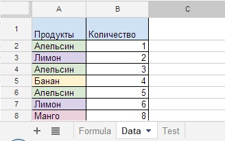
Figure 21
We have the initial data in the Data sheet (Figure 21), and the result on the Formula sheet in column D (Figure 22). Columns E, F, G show the arguments used in the formula, and column H shows a general view of the formula, which is in column D and calculates the result.

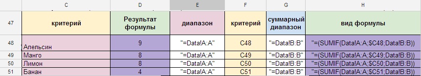
Figure 22
The example above shows a general view of how the “Sum If” formula works with one condition, but the most commonly used is “Sum IF” (with multiple conditions).

Summing cells IF, many conditions.

We continue to consider the problem with products at another level.
The party is just beginning, and after calling your friends, you begin to understand that there will not be enough alcohol. And you need to buy it. Each of your friends should bring a strong drink with them. You need to find out the number of bottles of beer that you need to bring and give a task to your friends.

• Description: sum of IF (with multiple conditions).
• Formula type: \u003d SUMIF (‘Data’! Range_1 & ‘Data’! Range_2; criteria_1 & criterion_2; ‘Data’! Total_range).
• The formula itself: \u003d (ARRAYFORMULA (SUMIF ((Data! E: E & Data! F: F); (B53 & C53); Data! G: G)))

We have the initial data on the Data sheet (Figure 23).

Figure 23
Suppose that on the Formula sheet, in cell B53 (criterion_1 \u003d Beer) there should be the name of the drink, and cell C53 (criterion_2 \u003d 2) is the number of friends who will bring Beer. As a result, cell D53 will contain the result that we need to buy 15 bottles of beer. (Figure 23.1) that is, the formula will determine the amount based on two criteria - beer and number of friends.

Figure 23.1
If there are more such positions, lines 16 and 21 (Figure 24), then the number of bubbles in column G is summed up (Figure 24.1).

Figure 24
Total:

Figure 24.1

Now let's give a more interesting example:

Ha ... the party continues, and you remember that you need a cake, but not easy, and super - mega cake, with different spices, which, as luck would have it, are also encrypted with numbers. The challenge is to buy the spices in the right number of bags of each spice. The chef encrypted the required amount in the table (Figure 25.1), columns A and B (in the adjacent columns we do our calculations).
Each spice has its own serial number: 1,2,3,4. (Figure 25).

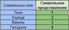
Figure 25
Our task is to count the number of repeated values, in our case, these are numbers from 1 to 4 in column B and determine the percentage of each of the spices.

• Description: Counting the number of identical digits in large arrays under additional conditions.
• Formula type: COUNT IF ('Formula'! Range_A55: A61 + 'Formula'! Range_B55: B61; ConditionA ”Spices” + ConditionB ”number from 1 to 4”; Sheet ”Formula '! Range_B55: B61) / ConditionB” number from 1 up to 4 ")

• The formula itself: \u003d ((ARRAYFORMULA (SUMIF ("Formula"! $ A $ 55: $ A $ 61 & "Formula"! $ B $ 55: $ B $ 61; $ F $ 55 & $ E59; "Formula"! $ B $ 55: $ B $ 61))) / $ E59)

We have the initial data in the range A55: B61, the selection condition is selected by cell F55 and E59: E62, and the result is in the range of cells F59: F62 (counting the number of repetitions of numeric values \u200b\u200bwhen conditions match).

• Description: Calculates the percentage of spices.
• Formula type: Amount * 100% / Total_amount
• The formula itself: \u003d F58 * $ G $ 56 / F $ 56

Figure 25.1
Ultimately, we have the number of repeats and the percentage.
To write the formula correctly, you must fully understand what you HAVE, what you WANT TO OBTAIN and in what form. You may need to change the look of the initial data for this.
Moving on to the next example

Counting values \u200b\u200bin merged cells.

If the formulas use values \u200b\u200bin "merged cells", then the first cell for the merged data is indicated, in our case it is column F, and cell F65 (Figure 26)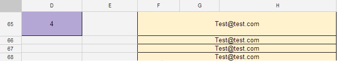



Figure 26.
And finally, we got to the worst formulas.

Counts the number of numbers in the argument list.

There are several types of such calculations, they are suitable for large tables in which you need to count the number of identical words or the number of numbers. But with the correct understanding of these formulas, you can work with them such miracles as, for example: counting words without taking into account the words of exceptions. See examples below.

• Description: Counts the number of cells containing numbers without text variables.
• Formula type: COUNT (value_1; value_2; ... value_30)
• The formula itself: \u003d COUNT (E45; F45; G45; H45)

We have the initial data in the range of cells E70: H70, and the result in cell D70 (Figure 27 - counting cells containing numeric values \u200b\u200bin a range that contains cells with text).

Figure 27.
Cells containing text and numbers are also not counted.

Figure 27.1.

Counting the number of cells containing numbers with text variables.

• Description: Counts the number of cells containing numbers with text variables.
• Formula type: COUNTA (value_1; value_2;… value_30)
• The formula itself: \u003d COUNTA (E46: H46)

We have the initial data in the range of cells E71: H71, and the result in cell D71 (Figure 28 - counting all values \u200b\u200bin the range).

Figure 28.
Also, the formula counts cells containing only punctuation marks, tabs, but does not count empty cells.

Figure 28.1

Substitution of values \u200b\u200bunder conditions.

• Description: Substitution of values \u200b\u200bunder conditions.
• Formula type: "\u003d IF (AND ((Condition1); (Condition2)); Result is 0, if conditions 1 and 2 are met; if not, then the result is 1)"
• The formula itself: "\u003d IF (AND ((F73 \u003d 5); (H73 \u003d 5)); 0; 1)"

We have the initial data in cells F73 and H73, and the result in cell D73 (If F73 \u003d 5 and H73 \u003d 5 then D73 \u003d 0 in all other cases 1) (Figure 29).

Figure 29.

Figure 29.1
Let's complicate the example.
Count the number of cells in which the time frame is written, excluding the words "auto answer", "busy", "-".

• Formula type: "\u003d COUNTA (Range_A) -COUNTIF (Range_A;" auto answer ") - COUNTIF (Range_A;" - ") - COUNTIF (Range_A;" busy ")"

• The formula itself: \u003d COUNTA ($ E74: $ H75) -COUNTIF ($ E74: $ H75; "auto reply") - COUNTIF ($ E74: $ H75; "-") - COUNTIF ($ E74: $ H75; "busy" )

We have the initial data in the range of cells E74: H75, and the result in cell D74 (Figure 30).

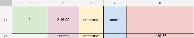
Figure 30
So we have come to the end of our little educational program on formulas in Google SpreadSheet and I have high hopes that I have shed light on some aspects of analytical work with formulas.
To be honest, the formulas were literally hard-won. Each of them has been created over time. I hope you enjoyed my article and the examples in it.
And finally, as a gift. And may the developers forgive me!

Formula "DOCUMENT KILLER".

If you need to hide a document from prying eyes forever, then this formula is for you.
The formula itself: "\u003d (ARRAYFORMULA (SUMIF ($ A: $ A & $ C: $ C; $ H: $ H & F $ 2; $ C: $ C)))". $ H: $ H governs the distribution of the formula. After you run the fomlula (Figure 31), below in the cells it will start multiplying the following CONTINUE function (cell; row; column).

Figure 31
The formula loops around the entire formula column. In order to kill a document, you need to try a little, create the N-th number of cells and write the formula in the first cells of the N-th number of columns. All! No one else can correct and check the document!
Here is what the google help page says about workload and limits -

Organization of calculations in spreadsheets, Relative reference, Absolute reference, Mixed reference, Built-in function, Logical function, Conditional function, Informatics Grade 9 Bosov, Informatics Grade 9

The main purpose of spreadsheets is to organize all kinds of calculations. You already know that:
- Calculation is the process of calculating by formulas;
- A formula begins with an equal sign and can include operation signs, numbers, references, and built-in functions. Let's first consider the issues related to the organization of calculations in spreadsheets.

3.2.1. Relative, absolute and mixed links
The reference indicates the cell or range of cells that you want to use in the formula. Links allow:
- use in one formula that are in different parts of the spreadsheet;
- use the value of one cell in several formulas. There are two main types of links:
1) relative - depending on the position of the formula;
2) absolute - not depending on the position of the formula.
The difference between relative and absolute references appears when you copy a formula from the current cell to other cells.
Relative links. A relative reference in a formula determines the location of the data cell relative to the cell in which the formula is written. When you change the position of the cell containing the formula, the reference changes.
Consider the formula \u003d A1 ^ 2 written in cell A2. It contains a relative A1 reference that is perceived table processor as follows: the contents of a cell that is one line higher than the one in which the formula is located should be squared.
When you copy a formula along a column and along a row, the relative reference is automatically adjusted like this:
- offset by one column leads to a change in the reference of one letter in the column name;
- an offset by one line leads to a change in the reference of the line number by one.
For example, when you copy a formula from cell A2 to cells B2, C2 and D2, the relative reference automatically changes and the above formula becomes: \u003d B1 ^ 2, \u003d C1 ^ 2, \u003d D1 ^ 2. When copying the same formula into cells AZ and A4, we get, respectively, \u003d A2 ^ 2, \u003d AZ ^ 2 (Fig. 3.4).

Example 1. In grade 8, we considered the problem of the population of a certain city, annually increasing by 5%. Let's calculate the estimated population of the city in the next 5 years in spreadsheets, if in the current year it is 40,000 people.
Let's enter the initial ones into the table, enter the formula \u003d B2 + 0.05 * B2 in cell OT with relative links; copy the formula from cell OT to the range of cells B4: B7 (Fig. 3.5).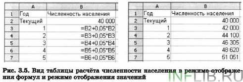



We (according to the condition of the problem) carried out the annual calculation of the population according to the same formula, the initial ones for which were always in a cell located in the same column, but one row higher than the calculation formula. When copying a formula containing relative references, the changes we needed were made automatically.
Absolute links. An absolute reference in a formula always refers to a cell at a specific (fixed) location. In an absolute reference, a $ is placed before each letter and number, for example $ A $ 1. Changing the position of the cell containing the formula does not change the absolute reference. When copying a formula along lines and along columns, the absolute reference is not adjusted (Fig. 3.6).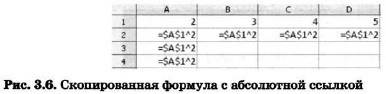

Example 2. A certain citizen opens an account in the bank for 10,000 rubles. He was informed that every month the amount of the deposit would increase by 1.2%. In order to find out the possible amount and the increment of the deposit amount after 1, 2, ..., 6 months, the citizen made the following calculations (Fig. 3.7).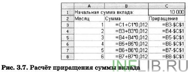

Mixed links. A mixed reference contains either an absolutely addressable column and a relatively addressable string ($ A1), or a relatively addressable column and an absolutely addressable string (A $ 1). When you change the position of the cell containing the formula, the relative part of the address changes, but the absolute part of the address does not change.
When copying or filling in a formula along the rows and along the columns, the relative reference is automatically adjusted, and the absolute reference is not adjusted (Figure 3.8).

To convert a link from relative to absolute and vice versa, you can select it in the input line and press F4 (Microsoft Office Excel) or Shift + F4 (OpenOffice.org Calc). If you select a relative reference, such as A1, then the first time you press this key (key combination), both the row and the column will be set to absolute references ($ A $ 1). On the second click, only the string (A $ 1) will get the absolute link. On the third click, only the column ($ A1) will get an absolute reference. If you press the F4 key (the Shift + F4 key combination) again, then relative links (A1) will be established for the column and row again.
Example 3. It is required to compile a table for adding the numbers of the first ten, that is, to fill in a table of the following form: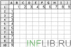

When filling in any cell of this table, the corresponding values \u200b\u200bof the cells of column A and row 1 are added up. In other words, the first term remains unchanged the name of the column (you should give an absolute reference to it), but the row number changes (you should give a relative reference to it); the second term changes the column number (relative reference), but the row number (absolute reference) remains unchanged.
Enter in cell B2 the formula \u003d $ A2 + B $ 1 and copy it to the entire range B2: J10. You should have an addition table that every first grader will be familiar with.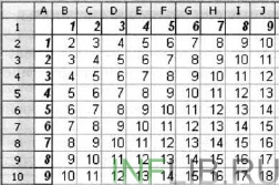


3.2.2. Built-in functions
When processing data in spreadsheets, you can use built-in functions - predefined formulas. The function returns the result of performing actions on the values \u200b\u200bthat act as arguments. Using functions allows you to simplify formulas and make the calculation process clearer.
Several hundred built-in functions are implemented in spreadsheets, divided into: mathematical, statistical, logical, textual, financial, etc.
Each function has a unique name that is used to call it. The name is usually the natural language abbreviation of the function name. When performing tabular calculations, the following functions are often used:
SUM (SUM) - sum of arguments;
MIN (MIN) - determination of the smallest value from the list of arguments;
MAX (MAX) - determine the largest value from the list of arguments.
The Function Wizard dialog box simplifies the creation of formulas and minimizes typos and syntax errors. When you enter a function into a formula, the Function Wizard dialog box displays the function name, all its arguments, a description of the function and each of the arguments, the current result of the function and the entire formula.
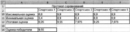
Example 4. The rules of refereeing in international competitions in one of the sports are as follows:
1) the performance of each athlete is evaluated by N judges;
2) the maximum and minimum marks (one, if there are several) of each athlete are discarded;
3) the arithmetic mean of the remaining marks is taken into account for the athlete.
Information about the competition is presented in the spreadsheet:



It is required to calculate the marks of all participants in the competition and determine the winner's mark. For this:
1) in cells А10, A1, А12 and А14 we enter the texts "Maximum mark", "Minimum mark", "Final mark", "Score of the winner";
2) in cell B10 we enter the formula \u003d MAX (OT: B8); copy the contents of cell B10 to cells C10: F10;
3) in cell В11 we enter the formula \u003d MIN (ВЗ: В8); copy the contents of cell B10 to cells C11: F11;
4) in cell B12 we enter the formula \u003d (SUM (OT: B8) -B10-B11) / 4; copy the contents of cell B12 to cells C12: F12;
5) in cell B14 we enter the formula \u003d MAKC (B12: F12).

3.2.3. Logic functions
In the study of the previous material, you have repeatedly come across logical operations NOT, AND, OR (NOT, AND, OR). You used the logical expressions built with their help when organizing searches in databases, when programming various computing processes.
Boolean operations are also implemented in spreadsheets, but here they are presented as functions: the name is written first logical operationand then the logical operands are listed in parentheses.
For example, a boolean expression corresponding to the double inequality 0<А1<10, в электронных таблицах будет записано как И(А1>0; A1<10).
Remember how we wrote a similar logical expression when we got acquainted with databases and the Pascal programming language.
Example 5. Let's calculate in spreadsheets the values \u200b\u200bof the logical expression NOT A AND NOT B for all possible values \u200b\u200bof the logical variables included in it.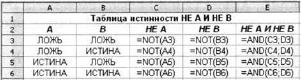

In solving this problem, we followed the well-known algorithm for constructing a truth table for a logical expression. Calculations in the ranges of cells SZ: C6, D3: D6, EZ: E6 are carried out by a computer according to the formulas we have specified.

To check conditions when performing calculations in spreadsheets, a logical IF function is implemented, called a conditional function.
The conditional function has the following structure:
IF A (<условие>; <действие1>; <действие2>)
Here<условие> - a logical expression, that is, any expression built using operations and logical operations that takes the value TRUE or FALSE.
If the boolean expression is true, then the value of the cell in which the conditional function is written is determined<действие1>if false -<действие2>.
What reminds you of a conditional function?
Example 6. Consider the problem of admission to a school basketball team: a student can be accepted into this team if his height is at least 170 cm.
Information about the applicants (name, height) is presented in a spreadsheet.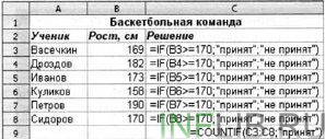

Using a conditional function in the range of cells СЗ: С8 allows you to make a decision (accepted / not accepted) for each applicant.
The COUNTIF function allows you to count the number of cells in a range that meet a specified condition. This function calculates the number of applicants selected for the team in cell C9.

writing mathematical formulas

General characteristics and launch of the formula editor

Writing and editing formulas in Word is carried out using the formula editor MicrosoftEquation3.0, which contains about 120 templates. It allows you to insert mathematical signs and expressions into your document, including fractions, powers, integrals, etc. When you write a formula, the appropriate styles are automatically applied for its various components (reduced font size for exponents, italics for variables, etc.).

Example. Launching the formula editor.

1. Place the cursor at the place where you enter and edit the formula.

2. In the menu Insertset the command An object…, open the dialog box Inserting an Object.

3. On the tab Creaturein field Object type:let's choose MicrosoftEquation3.0.

4. Click on the OK button.

This will open a dialog for working with the formula editor.

The formula editor is launched to edit an existing formula by double-clicking in the formula field.

Completion of editing or writing a formula is done outside of the formula entry box.

Formula editor interface

After starting the formula editor, the formula editor window will open, which has its own toolbar. This panel consists of two rows of buttons:

 access to character sets,

 access to sets of templates.

You can enter letters of the Russian and Latin alphabets into the formula from the keyboard, as well as signs of the simplest mathematical operations (+, -, /).

The line of buttons for accessing character sets allows you to enter mathematical symbols (operation signs and letters of the Greek alphabet) into the formula.

The following character sets are located in the top line of the toolbar from left to right:

 Symbols of relations;

 Intervals and dots;

 Mathematical differences;

 Signs of operations;

 Arrow symbols;

• Symbols of set theory;

 Logical signs;

 Various symbols;

 Greek letters.

Using the toolbar templates, you can insert signs of a number of mathematical operations into the formula, set the symbols of integrals, sums, products. In addition, templates allow you to set the form of a mathematical expression (fraction, degree, index, matrix, etc.) for the subsequent input of mathematical symbols into the workpiece obtained using the template.

The following sets of templates are located in the bottom row of the toolbar from left to right:

 Templates of constraints;

 Templates of fractions and roots;

 Creation of sub and superscripts;

 Integrals;

 Overlines and underlines;

 Marked arrows;

 Works and templates of set theory;

 Matrix templates.

When typing formula characters, the cursor is in the form of “or” characters. The character entered in the formula is placed to the right or left of the vertical bar and above the horizontal line of the input cursor.

Writing and editing formulas

When writing and editing a formula, the next character can be entered at its end into the main input line - the place of the character being entered is automatically marked with a slot (a rectangle with a dashed line). If you need to enter a symbol for a sum, integral or other complex formula structure, you should use the mouse to select the corresponding icon in the appropriate set of templates.

Blanks obtained with templates can be inserted in the middle of the slot. Thus, multi-step formulas are created.

Editing an existing formula involves deleting its individual elements and entering new ones using the formula editor.

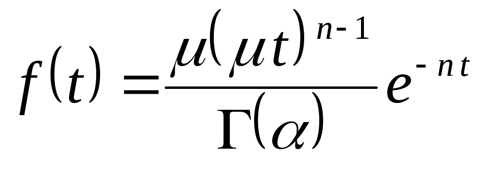
Example. Writing a fragment of a formula.

Let's introduce a fragment of a formula of the form: .

1. Click to open a submenu with a set of sum templates.

2. Select the sum template with upper and lower limits (in the upper row, the rightmost template) by clicking the mouse.

As a result, a blank of the form will appear in the formula editing window: .

3. Let's enter the required symbol, number or expression in each of the slots, after placing the input cursor there, and the fragment of the formula will take the desired form.

Example. Deleting a Formula Element.

1. Select the element to be deleted by clicking the mouse.

2. Press the key .

If a formula element is a part of a fragment created using a template, then after deleting it, an input slot. An input slot can only be deleted together with the template to which it belongs.

In some cases, after deleting the elements of the formula, the graphic display of some of its remaining elements may be broken. To restore the formula to its normal appearance, run the command Redrawmenu View.

Example. Inserting new items into a formula.

1. Place the insertion cursor at the desired location in the formula.

2. Let's introduce the required sequence of symbols.

3. If necessary, using a template, insert a blank, and then fill its slots with the necessary symbols.

Example. Writing a formula with a fraction line.

.

1. Place the cursor at the location of the formula.

3. In the slot for entering the formula using the keyboard, type the beginning of the formula "

».

4. In the set Fraction and root patternsclick on the template

(top left template).

This will insert a template with two slots in the numerator and in the denominator of the fraction.

5. Into the denominator slot, enter the expression

, and in the numerator slot -

.

6. In a set of templates Creating subscripts and superscriptsselect the template that specifies the creation of the top right index.

7. In the slot that appears, enter the expression for the degree "n-1".

8. Place the cursor at the end of the already typed part of the formula.

9. In a set of templates Creating subscripts and superscriptschoose a template.

10. In the appeared blank in the main slot, enter the symbol “ e", And in the slot of the right superscript we enter the expression of the degree" - nt».

By clicking outside the formula box, close the formula editing dialog.

Writing matrix formulas

To write matrix formulas in the bottom line of the toolbar, there is a set Matrix templates.

Example. Writing a formula with curly braces.

Consider writing a formula of the form:

2. Open the formula editor window.

3. In the slot for entering the formula from the keyboard, enter “ y= ».

4. In the set Delimiter templatesclick on the template.

This will insert a curly brace with a slot to the right of it.

5. Place the cursor in the named slot.

6. In the set of Matrix templates, select the template:.

As a result, the slot to the right of the curly brace is converted to two slots located one above the other. This will proportionally increase the size of the curly brace itself.

7. Into the upper and lower slots, enter the corresponding formula expressions.

8. Close the formula creation dialog by clicking the mouse.

Example. Writing a matrix formula.

Consider an example of writing the formula for the determinant of the 3rd order:

.

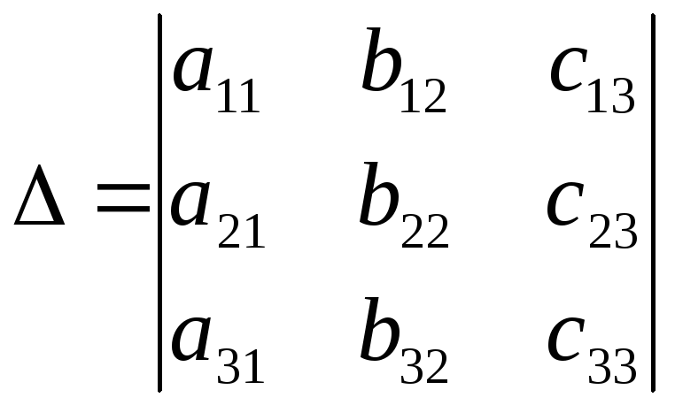1. Place the cursor at the location of the formula.

2. Open the formula editor window.

3. In the slot of the frame for entering the formula from the keyboard, enter " \u003d".

4. Open the set Matrix templatesand select a template:

5. A dialog box will open The matrix... Let's set the number of rows and the number of columns of the matrix.

6. By clicking the mouse to the left and right of the matrix image in the window, set the vertical lines along the matrix edges.

7. In the group of switches Column alignmentselect the switch Center.

8. In the Row alignment radio button group, select the radio button On the main line... Click OK.

This will insert a matrix blank with three rows and three columns and vertical lines on the sides.

9. In the first slot of the first line, enter the symbol “ and».

10. In the set of templates Create sub and superscripts, select the template that specifies the creation of the lower right index.

11. Introduce "11" into it.

12. Fill the rest of the slots in the same way.

13. By clicking outside the formula box, close the formula creation dialog.

Resizing and moving a formula

Resizing and moving the formula is done right in the main window of the Word document. Before performing any of these actions, the formula must be selected with a mouse click.

Example. Resizing a formula.

1. Select the formula by clicking the mouse.

2. Place the mouse pointer on one of the eight handles of the selection box and drag it until you get the desired size.

If you change the size of the formula disproportionately, the relative position of the elements may be violated.

To change the scale of the formula, select the formula and select Edit | Object | Formula | Open... Then select the appropriate scale (25% to 400%) from the menu View.

Example. Move the formula.

1. Select the formula by clicking the mouse.

2. Move the mouse pointer over the formula so that it takes the form of an arrow directed to the left.

3. Press the left mouse button and drag the formula to the desired location in the document.

4.To change the horizontal position of the formula, set the command Paragraph…menu Formatand set the required values \u200b\u200bfor the parameters of the paragraph with the formula.

This is a chapter from the book: Michael Girwin. Ctrl + Shift + Enter. Mastering array formulas in Excel.

This post is for those who are really interested in complex array formulas. If you just need to retrieve a list of unique values \u200b\u200bonce, it's much easier to use an Advanced Filter or PivotTable. The main advantages of using formulas are automatic updates when changing / adding source data or selection criteria. Before reading, it is advisable to brush up on the ideas contained in the previous materials:

• (chapter 11);
• (chapter 13);
• (chapter 15);
• (chapter 17).

Figure: 19.1. Retrieving Unique Records Using Option Advanced filter

Download a note in format or, examples in format

Retrieving a unique list from one column using an option Advanced filter

In fig. 19.1 shows a dataset (range A1: C9). Your goal is to get a list of unique racing tracks. Since you need to keep the original data, you cannot use the option Remove duplicates (menu DATA –> Work with the data –> Remove duplicates). But you can use Advanced filter... To open a dialog box Advanced filter, go through the menu DATA –> Sort and filter –> Additionally, or press and hold the Alt key, and then press S, L in sequence (for Excel 2007 or later).

In the opened dialog box Advanced filter (fig.19.1) set the option copy the result to another location, check the checkbox Unique records only, specify the region to retrieve unique values \u200b\u200bfrom ($ B $ 1: $ B $ 9) and the first cell where the retrieved data will be placed ($ E $ 1). In fig. 19.2 shows the resulting unique list (range E1: E6). If you don't include the field name in Original Range dialog box Advanced filter (instead of using $ B $ 2: $ B $ 9 in Figure 19.1) Excel will treat the first row of the range as a field name, and you risk getting a duplicate. In fig. 19.3 shows one of many possible uses for a unique list.

Retrieve a unique list based on a criterion with an option Advanced filter

In the last example, you retrieved a unique list from one column. An advanced filter can also retrieve a unique set of records (that is, the entire source table rows) using a criterion. In fig. Figures 19.4 and 19.5 show a situation in which you need to extract unique records from the range A1: D10, for which the company name is ABC. Later in this chapter, you will see how to do this job using a formula. However, if you don't need the process to be automatic, you can use Advanced filter, which is certainly simpler than the formula.

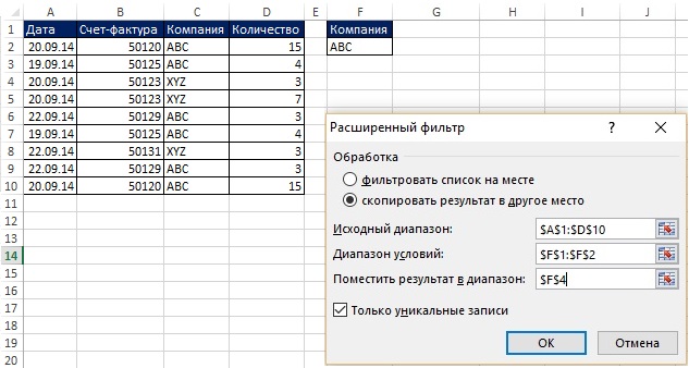
Figure: 19.4. You need unique records for an ABC company; to enlarge the image, right-click on it and select Open picture in a new tab

Figure: 19.5. Using Advanced filter to retrieve unique records based on criteria is much easier than the formula method. However, the retrieved records will not be automatically updated if the criteria or source data changes.

Retrieving a Unique List from a Single Column Using a Pivot Table

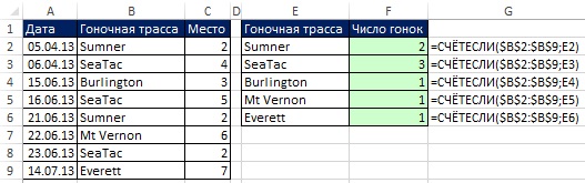
If you are already using pivot tables, then you know that every time you put any field in the area Strings or Columns (Figure 19.6), you will automatically get a unique list. In fig. Figure 19.6 shows how you can quickly create a unique list of racetracks, and then count the number of visits to each of them. While a pivot table is useful for retrieving a unique list from a single column, it is unlikely to be useful for retrieving unique records based on criteria.

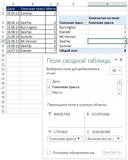
Figure: 19.6. You can use summary tablewhen you need a unique list and subsequent calculation based on it

Extract unique list from one column using formulas and helper column

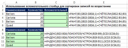
Using a helper column makes retrieving unique data easier than using array formulas (Figure 19.7). This example uses the techniques you learned in (using the COUNTIF function) and (using a helper column). If you now change the original data in the B2: B9 range, the formulas will automatically reflect these changes in the D15: D21 area.

Array Formula: Retrieve a Unique List from a Single Column Using the SMALL function

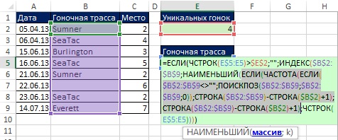
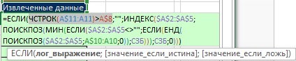
Since the array formulas used in this section are quite complex to understand, their creation is broken down into stages: the first is a fragment that counts unique values \u200b\u200b(Chapter 17); the second is criteria-based data extraction (Chapter 15). In fig. Figure 19.8 shows the formula for calculating unique values \u200b\u200b(since this is an array formula, you can enter it by pressing Ctrl + Shift + Enter). Note the following aspects of this formula:

1. The FREQUENCY function returns an array of numbers (Fig. 19.9): for the first appearance of a race track, the number of its occurrences in the original data is returned; for each subsequent occurrence of the race track, zero is returned (see). For example, Sumner appears at the first and fifth positions in the array. In the first position, the FREQUENCY function returns 2 - the total number of Summer in the range B2: B9, in the fifth position - 0.
2. The FREQUENCY function is located in the argument log_expression the IF function, so the IF function returns TRUE for any nonzero value, and FALSE for any nonzero value.
3. Argument value_if_true of the IF function contains 1, so the SUM function counts the number of such ones.

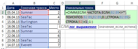
Figure: 19.8. The FREQUENCY function is located in the argument log_expression functions IF

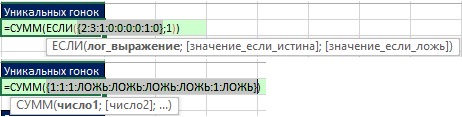
Figure: 19.9. (1) the FREQUENCY function returns an array of numbers; (2) the IF function returns 1 for nonzero numbers, and FALSE for zeros

Now let's create a formula for retrieving a unique list. In fig. 19.10 shows an array of relative positions placed in an argument array functions SMALL.

In the previous example (Fig. 19.9) in the argument value_if_true the IF function had one allocated, so the IF function returned one and FALSE. Here (fig.19.10) the argument value_if_true contains: LINE ($ B $ 2: $ B $ 9) -LINE ($ B $ 2) +1. Therefore, the IF function (inside the SMALL function) returns a relative position number in a range with a unique race track, or FALSE for takes (Figure 19.11).

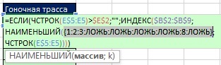
Figure: 19.11. IF function returns a relative position number in a range with a unique race track, or FALSE for takes

In fig. 19.12 show the results of the formula. In fig. 19.13 shows that as soon as the initial data changed, the formulas immediately reflected these changes. But what if you add new entries? Next, you will see how to create dynamic range formulas.

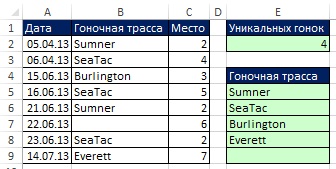
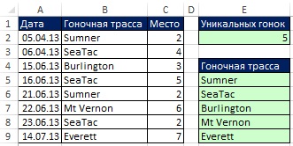
Figure: 19.13. If the original data changes, the formula updates immediately. Filter and Advanced Filter cannot update automatically without writing VBA code

Array formula: extract a unique list from a single column using dynamic range

Let's add last example by what you've learned about formulas that use specific names based on dynamic range (). In fig. 19.14 is the formula for determining the name Track... This formula assumes that you never enter a record after line 51.

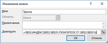
Figure: 19.14. Name definition Track based on formula

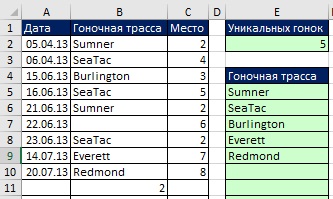
Once you've identified the name, you can use it in any formula. In fig. Figure 19.15 shows how to use a name to count the number of unique values \u200b\u200b(compare with Figure 19.8). And in fig. 19.16 shows a formula that extracts the unique values \u200b\u200bthemselves from a list of race tracks. Note that instead of snippet range<>"" (As it was in Fig. 19.8 and 19.10), the function ETEXT is used (any text will return TRUE). When using ETEXT, if you enter a number (as in cell B11), or any other non-text, the formula will ignore that value. In fig. 19.17 shows that the formula will automatically extract any new trace names, ignoring the numbers.

Figure: 19.16. Retrieving a Unique Alignment Name Based on Dynamic Range

Create a Unique Values \u200b\u200bFormula for a Dropdown List

Based on the example just seen, let's define a middle name - TrackList, also based on dynamic range, but now referring to a list of unique traces (range E5: E14, Figure 19.18). Since the range E5: E14 contains only text and empty values \u200b\u200b(test strings of zero length - ""), in the argument lookup_value the MATCH function can use wildcards *? (which means at least one character). And in the argument match_type the MATCH function should use a value of –1 to find the last text element in a column that contains at least one character. As shown in fig. 19.18, then you can use a specific name in the field A source window Validating Input Values (for more details on creating a drop-down list, see). The dropdown list can expand and contract as new data is added or removed in column B.

Where wildcards are to be treated like regular characters

As you learned in, sometimes wildcards have to be treated as symbols. In fig. 19.18 shows how you can change the formulas for such cases. You append a tilde before the argument range lookup_value SEARCH function and append an empty string to the back of the range in the argument lookup_array.

Using a helper column or array formula to retrieve unique records based on criteria

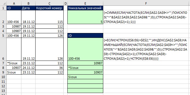
At the beginning of this post, it was shown that for retrieving unique records based on criteria, it works great Advanced filter... However, if you need an instant update, you can use the helper column (Figure 19.20) or array formulas (Figure 19.21).

Dynamic formulas to extract customer names and sales

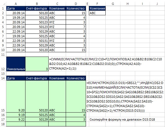
The formulas are shown in Fig. 19.22. For example, if you add a new entry TTTrucks on line 17 , the SUMIF formula in cell F15 will automatically add the new value. If you add a new customer in column B, it will immediately appear in column E, and the SUMIF formula in column F will show the new total.

Figure: 19.22. Using a specific name and two array formulas to retrieve unique customers and sales

Note that the SUMIF function in the argument sum_rangecontains one cell - $ C $ 10. Here's what the SUMIF formula help has to say on this topic: argument sum_range may not be the same size as the argument range... The top-left cell of the argument is used as the starting cell when determining the actual cells to be added sum_range, and then the cells of the part of the range corresponding in size to the argument are summed range... Formulas entered in cells E15 and F15 are copied along the columns.

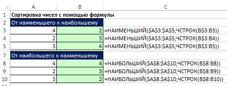
Sorting numeric values

The formulas for sorting numbers are pretty simple, but for sorting mixed data they are insanely complex. Therefore, if you do not need an instant update, then it is better to do without formulas by using the option Sorting... In fig. 19.23 shows two sorting formulas.

In fig. 19.24 shows how you can use a helper column to sort numbers. Since the RANK function does not sort the same numbers (giving them the same rank), the COUNTIF function has been added to distinguish them. Note that the COUNTIF function has an extended range that starts one line up. This is necessary so that the first appearance of any number does not contribute. The second appearance of the number will increase the rank by one. This sequential numbering sets the order in which the INDEX and SEARCH functions retrieve records in the A8: B12 range.

If you can afford to create an auxiliary column in the data extraction area (range A10: A14 in Figure 19.25), it is convenient to apply the above-described sorting of numbers based on the SMALL function, and based on it, extract the names using the array function.

Figure: 19.25. If you cannot use a helper column, apply the SMALL sort (in cell A11) and an array formula (in cell B11)

Often in business and sports it is required to extract the N best values \u200b\u200band the names associated with those values. Start the solution with the COUNTIF formula (cell A11 in Figure 19.26), which will determine the number of records to display. Note that the argument criterion in the COUNTIF function in cell A11 - more or equal the value in cell D8. This allows you to display all boundary values \u200b\u200b(in our example, although you want to display Top 3, there are four suitable values).

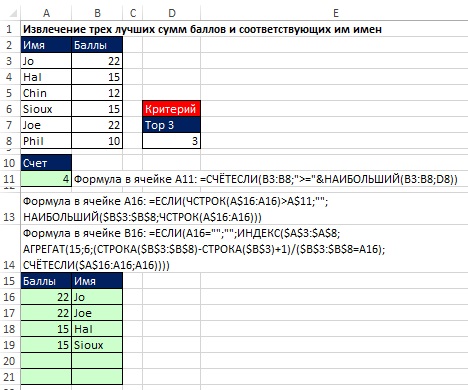
Figure: 19.26. Retrieving the top three scores and their corresponding names. When N changes in cell D8, the area A15: B21 will be updated

Sorting text values

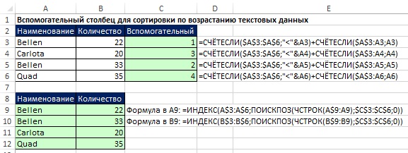
If you can use an auxiliary column, the task is not so difficult (Figure 19.27). Comparison operators process text characters based on the numeric ASCII codes assigned to the characters. In cell C3, the first COUNTIF function returns zero, and the second adds one. In C4: 2 + 1, C5: 0 + 2, C6: 3 + 1.

Sorting mixed data

The formula that allows you to extract unique values \u200b\u200bfrom mixed data and then sort them is very large (Figure 19.28). In its creation, ideas were used that were encountered earlier in this book. Let's start exploring the formula by looking at how the standard Excel sort function works.

Excel sorts the results in the following order: numbers first, then text (including zero-length strings), FALSE, TRUE, error values \u200b\u200bin the order in which they appear, blank cells. All sorting is done in accordance with ASCII codes. There are 255 ASCII codes, each of which corresponds to a number from 1 to 255:

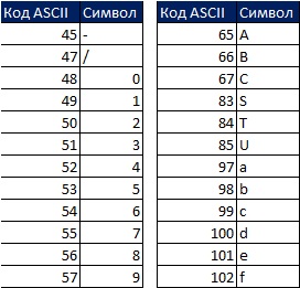
For example, 5 is ASCII 53 and S is ASCII 83. If you sort the two values, 5 and S, from lowest to highest, then 5 is higher than S because 53 is less than 83.

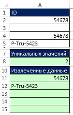
The data set in the A2: A5 range (Fig. 29) is converted to the E2: E5 range in accordance with the sorting rules. To better understand sorting principles, consider the values \u200b\u200bin the range C2: C5. For example, if you ask the question "How much above me in rank?" to the ID in cell A2 (54678), the answer will be zero, because in the sorted list, ID 54678 will be the topmost. SD-987-56 will have three IDs above it. You need a formula to get values \u200b\u200bin the range C2: C5.

First, select the range E1: H1 and in the formula bar, type \u003d TRANSPOSE (A2: A5), enter the formula by pressing Ctrl + Shift + Enter (Fig. 19.30). Next, select the range E2: H5 in the formula bar, type \u003d A2: A5\u003e E1: H1 and enter the formula by pressing Ctrl + Shift + Enter (Fig. 19.31). In fig. Figure 19.32 shows the result as a rectangular array of TRUE and FALSE values \u200b\u200bthat correspond to each of the cells in the resulting array, as the answer to the question "Is the row heading greater than the column heading?"

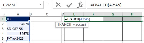
Figure: 19.30. Select the range E1: H1 and enter array formulas

Figure: 19.31. In the range E2: H5, enter the array formula \u003d A2: A5\u003e E1: H1

Figure: 19.32. Each cell of the range E2: H5 contains the answer to the question "Is the row heading larger than the column heading?"

For example, cell E3 asks the question: SD-987-56\u003e 54678. Since 54678 is smaller than SD-987-56, the answer is TRUE. Note that the range E3: H3 includes three TRUE and one FALSE values. Looking back at fig. 19.29, you can see that the number three is in cell C3.

As shown in Figures 19.33 and 19.34, you can convert TRUE and FALSE values \u200b\u200bto ones and zeros by adding double negatives to the array formula. Since the original array (E2: H5) has a dimension of 4 × 4, and you want the result in the form of a 4 × 1 array, use the MULTIFUNCTION function (see Fig. 19.35 and). The MULTIPLE function is an array function, so enter it by pressing Ctrl + Shift + Enter (Figure 19.36). Now, instead of using the range E2: H5, add the appropriate elements inside the formula (Figure 19.37).

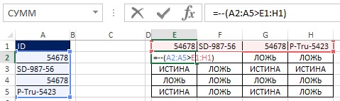
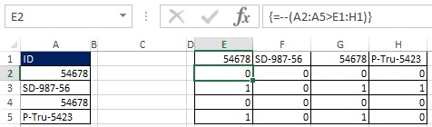
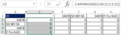
Figure: 19.36. By selecting the range C2: C5 and entering the array function MULTIPLE you get a column of numbers that say how many IDs are in the sorted list above the selected one

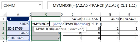
Figure: 19.37. Instead of using the auxiliary range E2: H5, the corresponding elements are added inside the formula

In fig. 19.38 shows how you can replace an array of constants with STRING ($ A $ 2: $ A $ 5) ^ 0.

Figure: 19.39. To deal with potential empty cells, all occurrences of A2: A5 should be supplemented with an IF (A2: A5<>"", A2: A5); the LINE function does not require such an addition, since the function works with the address of the cell, not its content

Since the final formula will be used elsewhere, you need to make all ranges absolute (Figure 19.40). In fig. 19.41 shows the resulting values.

Figure: 19.40. Ranges A2: A5 turned into absolute

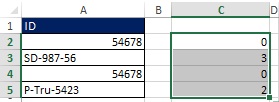
Since this element will be used twice in the future, you can save it under a specific name. As shown in the dialog box (Fig. 19.42), the formula is named SZB - How Many Values \u200b\u200bAre More.

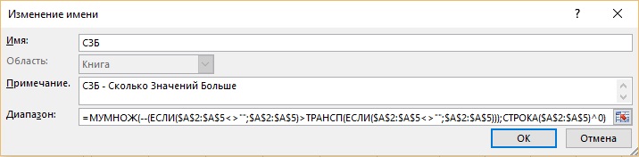
1. Argument array function INDEX refers to the original range A2: A5.
2. The first MATCH function will tell the INDEX function the relative position of the element in the A2: A5 array.
3. While the argument lookup_value the SEARCH function is left blank.
4. Specified name (SZB) in argument lookup_array will allow you to first access the element that has a value of 0, then 2, and finally 3.
5. Zero in argumentation match_type specifies an exact match, which will eliminate reference to duplicates.

Figure: 19.43. You start a formula to extract and sort the data in cell A11. Argument lookup_value the SEARCH function is left blank for now

Before you create an argument lookup_value function SEARCH, remember what, in fact, you need. There are three unique IDs that need to be sorted, so you need three numbers in the argument lookup_value as the formula is copied down. These numbers will allow you to find the relative position in the A2: A5 array, which you need to provide to the INDEX function:

1. In cell A11, the MATCH function will return 0, which corresponds to the relative position of 1 within the specified MSB name.
2. When the formula is copied down into cell A12, the MATCH function should return the number 2, and the relative position \u003d 4 within the MSB.
3. In cell A13, the MATCH function should return 3, and the relative position \u003d 2 within the MSB.

The picture emerges when you think about what the argument lookup_value when copying the formula down, the query must match: "Give the minimum value within a specific name of the SZB that has not yet been used." As shown in fig. 19.44 formula element MIN (IF (UND (SEARCH ($ A $ 2: $ A $ 5; A $ 10: A10; 0)); SZB)) returns the minimum value when you copy the formula down, answering the query exactly. The reason this works is because in the UNM fragment (SEARCH ($ A $ 2: $ A $ 5; A $ 10: A10; 0)) two lists are compared (see). Notice the expanding range A $ 10: A10 in the argument lookup_array... In cell A11, the combination of UND and MATCH helps to extract all unique numbers from the SZB and provide them to the MIN function. When you copy the formula down to cell A12, the ID that was extracted in cell A11 is again present in the extended range and will again be found in the range $ A $ 2: $ A $ 5. However, UND returns FALSE, and the value 0 is not extracted from the MWB. To see this, enter the array formula in Figure 19.44 by pressing Ctrl + Shift + Enter and copy it down.

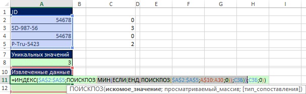
Figure: 19.44. Formula element in argument lookup_value function MATCH matches the query: "Give the minimum value within a specific SZB name that hasn't been used yet"

In fig. 19.45 shows that the argument lookup_array the second function SEARCH the range A $ 10: A10 has expanded to A $ 10: A11. To understand how this formula works, sequentially select its fragments and click on F9 (Fig. 19.46-19.49).

Figure: 19.45. Expandable range A $ 10: A11 now (in cell A12) includes the first ID (54678)

Figure: 19.46. The combination of the UND and the second SEARCH functions supplies an array of booleans; two FALSE values \u200b\u200bexclude null values \u200b\u200bfrom a specific MSB name

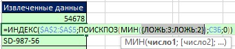
Figure: 19.47. Zeros are excluded and only numbers 3 and 2 remain; the number 2 is the minimum, so it is this that should be extracted as follows

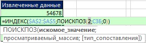
Figure: 19.48. The MIN function selects the number 2; now the MATCH function can find the correct relative position for the INDEX function

Figure: 19.49. The INDEX function will retrieve the value 2, which corresponds to the relative fourth position of the ID in the range A2: A5

Now, returning to cell A11, you can add another condition so that blank cells do not affect the formula (Figure 19.50).

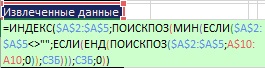
Figure: 19.50. There are two conditions inside the MIN function; first: "cells are not empty?", second: "value has not been used yet?"

In fig. 19.51 is the final formula. A condition has been added so that rows in the range A11: A15 remain empty after sorted unique values \u200b\u200bare retrieved. In fig. 19.52 shows what happens if cell A3 is made empty. Our addition to check for empty cells worked.

It wasn't easy. But, if you've read this far, I hope you enjoyed it.

CALCULATIONS IN ELECTRONIC TABLES

2.1. V o d f o r m u l s

The calculation of the cell value is done by entering a formula. Formulas always start with an equal sign “ = ”.

Formulas allow you to perform common mathematical operations on values \u200b\u200bfrom cells in a worksheet. For example, you need to add the values \u200b\u200bin cells B1 and B2 and display their sum in cell B5. To do this, place the cursor in cell B5 and enter the formula “\u003d B1 + B2”.

Formula input appears in both the table cell and the formula bar. When the button is pressed Enter calculations are performed and the result is obtained in the active cell.

The following operators can be used in formulas:

a r i f m e t i c e -

w a n i -

t e c t a -

& - concatenation of text values.

When calculating a formula in a table, the arithmetic order of operations is applied.

2.2. CREATION OF FORMULS WITH MUCH

You can enter cell coordinates in a formula by pointing the cursor at the desired cell. There is a risk of making a mistake when entering a formula manually. This can be avoided by acting as follows:

place the cursor in the cell where you want to enter the formula;

enter the equal sign “\u003d”;

place the cursor in the cell, the coordinates of which should be at the beginning of the formula, and click the mouse button;

enter an operator (for example, the “+” sign) or another character that continues the formula;

move the cursor to the cell whose coordinates you want to use in the formula and click the mouse button;

carry out these actions until the formula ends.

2.3. A b s o lute and about s and t e l n e c e c

There are three main types of addresses (links): relative, absolute and mixed.

The differences between relative and absolute references appear when you copy and move formulas from one cell to another.

When you move or copy, absolute links in formulas do not change, and relative links are automatically updated based on the new position.

For example, cell A1 contains a constant 4, cells B1 to B10 contain values \u200b\u200bfrom 0.1 to 1 in increments of 0.1. In order to get the result in cells D1: D10 according to the formula 4b i, where i \u003d 1, 2,…, 10, you need to type in cell D1 “\u003d $ A $ 1 * B1” and copy the formula into cells D2, D3,…, D10. In this case, D2 will contain the phrase “$ A $ 1 * B2”, in D3 - “$ A $ 1 * B3”, etc., where the content of $ A $ 1 does not change, since the address (link) is absolute, and B1 changes to B2, B3, ..., B10, since the address is relative.

To indicate the range of cells in formulas, use the symbol “ : ”, For example: A2 : A5.

To denote a group of non-adjacent cells, use the symbol “ ; ”, For example: A2; B5; E10.

2.4. EDITING FORMUL

Formulas are edited in the same way as the contents of cells.

Firstth way... You must select the cell you want, click on the formula bar and edit it.

Second way... Double-click a cell and edit the formula directly in the cell.

2.5. And using the function

One of the most useful features of EXCEL is its wide range of functions that allow you to perform various types of calculations. Each function has a syntax for writing:

FUNCTION NAME (argument 1; argument 2; ...).

Function arguments can be numbers, texts, logical values, error values, links, arrays. In decimal numbers, the integer part is separated from the fractional character “,”, for example: –30.003.

Text values \u200b\u200bmust be enclosed in double quotes. If the text itself contains double quotes, then they should be doubled.

Boolean values \u200b\u200bare TRUE and FALSE. Boolean arguments can also be comparison expressions for which TRUE or FALSE can be evaluated, for example: B10\u003e 20.

For example, the AVERAGE function calculates the arithmetic mean of a series of values. The expression “\u003d AVERAGE (6; 12; 15; 16)” will give the result 12.75. If the values \u200b\u200b6, 12, 15, 16 are stored in cells B10 - B15, then the formula can be written like this: “\u003d AVERAGE (B10: B15)”.

The SUM function is used to determine the sum of values, for example: “\u003d SUM (B10: B15)”. The numbers 6, 12, 15, 16 will be summed up.

It is convenient to introduce a function into a formula using Function Wizards ... The Function Wizard allows you to enter a function into the formula you are creating. To do this, do the following:

place the cursor in the cell where you want to enter the function;

in the standard toolbar, click the function wizard button ¦ x or execute the command Insert + Function ;

in the dialog box that appears in the list Categories select the desired function category. After that in the list Function the functions of the selected category appear;

in the list Function select a function and click on the button OK ;

a dialog box will appear depending on the type of function selected;

enter the desired values \u200b\u200bor cell ranges for the function arguments;

click on the button in the dialog box OK .

2.6. Auto matic s u m i r o n e

The simplest method for summing up a table is auto-summing. To do this, place the cursor in a cell below the column or to the right of the row, the values \u200b\u200bof which need to be summed up and click on the button of the standard toolbar Auto-summation (it shows the symbol “ å ”). Then press the button Enter .

When summing matrix elements by columns and rows, it is convenient to select the matrix cells with an additional row and column, and then press the button “ å ”. The sum of all rows and columns of the matrix will automatically be obtained.

2.7. F o rm uly for work with m a s i in a m i

Array formulas (tabular formulas) allow you to perform many calculations by writing a single formula. For example, you need to multiply the values \u200b\u200bin column A2: A6 by the corresponding B2: B6. Record the result in C2: C6 without copying the formula.

You need to do the following:

select the cells of the result C2: C6;

enter the “\u003d” sign;

select cells A2: A6;

enter the “*” sign;

highlight B2: B6;

press keyboard keys Shift + Ctrl + Enter .

The formula “(\u003d A2: A6 * B2: B6)” will be displayed in the formula bar, and the result will be obtained in all cells C2: C6.

Z A D A N I E 2

1) Run the EXCEL program.

2) In your own directory create a file named “lab_2.хls”.

3) Name the first sheet of the workbook “Lab. No. 2 (entering formulas) ”.

4) In cell A1 write your last name.

5) Create a report card according to the sample table. 2. Sum the items in each column and each row. Calculate the average score using formulas.

Table 2

	Maths	Economy	Informatics	Average score
Ivanov	5
Petrov	4
Sidorov	3
Yakovlev	4
Average score	4

6) Count the number of "5" marks in each subject. Print out a list of students with a GPA greater than “4”.

7) Compute y \u003d 2 x 2 + 3 x + 5, where the x argument changes from 0.1 to 1 in 0.1 increments. Use absolute references for constants 2, 3, 5, and relative references for x.

8) For a 4x4 matrix, calculate its determinant, its inverse matrix, square it and find the transposed matrix using table formulas.

9) Save the contents of the workbook.