Study of oscillations of a thread pendulum and measurement. Laboratory work in physics "study of the laws of a mathematical pendulum"
Study of the laws of a mathematical pendulum
Purpose of work: Study the laws of a mathematical pendulum and determine the acceleration of gravity
Equipment: Pendulum (ball on suspension), ruler, stopwatch or watch with second hand.
Brief theory:
A mathematical pendulum is an oscillator, which is a mechanical system consisting of a material point located on a weightless inextensible thread or on a weightless rod in a uniform field of gravitational forces.
The pendulum length l is the distance from the suspension point to the ball's center of gravity.
For a practical calculation of the oscillation period, use the formula:
 ,
,
where T is the oscillation period,
t - oscillation time,
n is the number of complete vibrations.
According to the laws of oscillation, the period of the pendulum can be determined by the formula:
 ,
,
The oscillation period of a mathematical pendulum does not depend on the mass of the ball.
P  the period of oscillation of a mathematical pendulum is directly proportional to the length of the pendulum and inversely proportional to the acceleration of gravity. This equation is called Huygens' formula.
History reference
Christian Huygens van Zuilichem (April 14, 1629 - July 8, 1695). Dutch physicist, mathematician, mechanic and astronomer and inventor. Born in The Hague. He studied law at Leiden University, but did not stop studying mathematics. Based on Galileo's research, he solved a number of problems in mechanics. In 1656, at the age of 27, he designed the first escapement pendulum clock. The creation of a clock that measured time with an unprecedented accuracy for that time had far-reaching consequences for the development of physical experiment and human practical activity. Before that, after all, time was measured by the outflow of water, burning of a torch or candle. The theory of oscillations created by Huygens by 1673 was one of the bases for later understanding the nature of light.
From the Huygens formula, by means of mathematical transformations, we obtain an expression for the acceleration of gravity:

A real model of a mathematical pendulum in our experiments will be a small ball suspended on a thin elastic thread. The size of the ball should be small compared to the length of the thread. This makes it possible to assume that all the mass is concentrated at one point, in the center of gravity of the ball.
Progress:
Determine the division price of devices:
ruler …… ..m / div.
stopwatch …… .s / div.
2. Determine the error of the instruments (the absolute error of the instruments is equal to ½ the scale interval):
ruler Δ l = …… ..m
stopwatch Δ t \u003d …… .s
Set the maximum length of the pendulum and measure it l 1 \u003d… .m.
Start the pendulum (deflection angle 10-15 0) and in time t count the number of vibrations n (at least 7).
By changing the number of vibrations, repeat the experiment 3 more times.
t 2 \u003d ………, n 2 \u003d …………. T 2 \u003d ………,
t 3 \u003d ………, n 3 \u003d …………. T 3 \u003d ………,
t 4 \u003d ………, n 4 \u003d …………. T 4 \u003d ………,
Change the length of the pendulum l 2 \u003d… .m and repeat all measurements.
Enter the data into the table.
№ measurements
Pendulum length
l, m
№ experience
Oscillation time,
t, s
The number of vibrations
n
Oscillation period,
T, s
Average value of the period, T avg, s
Free fall acceleration, g, m / s 2.
Mean
free fall acceleration, g average, m / s 2.
l cf \u003d
t Wed \u003d
relative: absolute:
![]() ,
,

Test questions:
How long is a mathematical pendulum with a period of 2 s?
Find the mass of the weight that, on a spring with a stiffness of 250 N / m, makes 20 vibrations in 16 s.
The acceleration of gravity on the Moon is 1.7 m / s 2. What will be the period of oscillation of the mathematical pendulum on the Moon, if on Earth it is equal to 1 s? Does the answer depend on the weight of the cargo?
The coordinate of the oscillating body changes according to the law x \u003d 0.5sin 45πt. What are the amplitude and period of oscillations?
The amplitude of continuous oscillations of the point is 12 cm, the linear frequency is 14 Hz, the initial phase of the oscillations is 0. Write the equation of motion of the point x \u003d x (t).
Scale division
Difference (without regard to sign) between values physical quantitycorresponding to the scale marks limiting division. In digital devices, the step of discreteness serves as a characteristic that replaces the scale division value.
a) select the two nearest digitized lines on the scale;
c) the difference in values \u200b\u200b(subtract the smaller from the larger) for the selected strokes, divide by the number of divisions.
H  this figure shows a thermometer scale on a large scale. We will use it to illustrate the rule for calculating the division price.
a) select the digitized strokes 20 ° С and 40 ° С
b) 10 divisions (gaps) between them
c) calculate: (40 ° С - 20 ° С): 10 divisions \u003d 2 ° С / div.
Answer: the price of divisions \u003d 2 ° С / div,
Digital devices do not have a scale explicitly, and instead of the division price, the price of the unit of the least significant digit of the number in the reading of the device is indicated on them.
P 
example:
1) the scale division price of this device is 1 (conventional units) / div.
2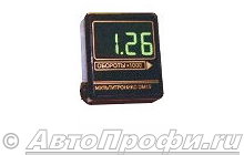
) the scale division of this device is 0.01 (conventional units) / div.
3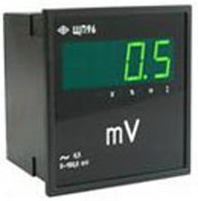
) the scale division of this device is 0.1 (conventional units) / div.
4) the scale division of this device is 0.001 (conventional units) / div.

I. purpose of work
Observations of the oscillatory movements of a mathematical pendulum, implemented on a device, the functional diagram of which is shown in Figure 1.
Measurement of the oscillation period of the pendulum at different lengths and amplitudes.
Determination of the mode of isochronism of oscillations of a mathematical pendulum.
Calculation of the gravitational acceleration of the ball from the results of the specified measurements.
II ... Theoretical part
Consider a device consisting of a small ball attached to a fixed point of the suspension using a weightless inextensible thread of a certain length (Fig. 1).
If the size of the ball is much less than the lengthl threads, then the ball can be seen as material point; and if the mass of the ball is much greater than the mass of the thread, then the latter can be considered weightless. The thread can also be considered inextensible provided that the gravity of the ball causes an infinitesimal elongation of the thread.
This device allows you to simulate the oscillatory motion of the so-called mathematical pendulum.
Figure: 1. A device for studying oscillations of a mathematical pendulum: 1. A metal plate for setting the angle of deflection of the pendulum; 2. Movable platform; 3. Measuring ruler.

Fig 2. Illustration of oscillatory movements of a mathematical pendulum.
Indeed, in the initial state, the thread is directed vertically downward (position 1 in Figure 2). In this case, the strengthF thread tension and strengthmg the ball's weights coincide with the direction of the thread, but oppositely directed. Since the thread is inextensible, both forces balance each other, i.e.F \u003d mg ... The ball is at rest. This state of the pendulum is called its equilibrium position.
Let's take the pendulum out of its equilibrium position by deflecting the ball from its initial state by an angleφ 0 (fig. 2). Then let go of it without pushing. By gravitymg the ball will begin to move towards the equilibrium position, after a while it will pass it, then on the other side of the equilibrium position it will deviate from it by some angle less thanφ 0 and, under the action of gravity, will again rush towards the equilibrium position. In the absence of external influences on the ball, the latter will perform the described movement in one plane. Obviously, the trajectory of the ball will be a circular arc of radiusl ... These movements are called vibrations.
Due to the action of the resistance force on the ball, its oscillations will be damped, which is evidenced by the fact that after each passage of equilibrium it will deviate from it at an ever smaller and smaller angle. However, if this process is observed for a fairly short time, then the oscillatory process can be recognized as continuous.
Consider the forces that act on the ball at an arbitrary timet. Let φ - the angle of deflection of the thread at this moment. We write the following equation of Newton's second law in the directionτ coinciding with the tangent drawn to the point of the trajectory of the ball, in which it is at the considered moment of timet.
ma τ \u003d - mg sin φ (1)
Here a τ - tangential acceleration,m Is the mass of the ball. The minus sign on the right in (1) takes into account the fact that when moving from the equilibrium position upwards, the force of gravity prevents this movement.
The angular acceleration ε of the ball is defined as the second time derivative of the angleφ, i.e.
. (2)
Between tangential accelerationa τ and angular ε there is an obvious connection
(3)
Equation (1) taking into account formulas (2) and (3) takes the form:
. (4)
In equation (4), the unknown functionφ (t) stands under the sign of the second-order derivative. Such an equation in mathematics is called an ordinary differential equation of the second order.
It can be simplified if we take into account that at small anglesφ, measured in radians. Then instead of (4) we will have
. (5)
Equation (5) describes the movement of the pendulum. It is also called the harmonic oscillator equation.
By direct substitution, one can verify that the solution of equation (5) has the form
, (6)
if we denote by
. (7)
Thus, it can be seen that changes in the angleφ in time occurs according to a sinusoidal law. The quantityφ 0 , equal to the maximum angle of deviation from the equilibrium position is called the amplitude of harmonic vibrations. The magnitude of the amplitude in this case depends on the initial deviation. The value under the sine sign is called the phase. The phase grows in proportion to time. The value under the sine sign is called the initial phase, which is zero in the considered motion.
The sine function, which determines the nature of the oscillatory movements, is a periodic function with a period equal to. The latter means that if afterT designate the period of oscillation of the pendulum, then we can write the following equality for the value of the phase
, (8)
where is the circular frequency.
Now taking into account (7) for the periodWe will have:
(9)
Relation (9) indicates that the linearization of equation (4) led to equation (5), the solution of which admits the independenceT on the amplitude φ 0.
Such fluctuations are called isochronous.
Formula (9) can also be represented as follows:
k l, (10)
where through
(11)
the slope of the linear functional dependence of the functionT 2 from argument l.
Consequently, the isochronism of the pendulum oscillations is verified by the validity of relation (10) according to the measured values \u200b\u200bof the periodT at different valuesl related to the same angleφ 0 .
The functional dependence constructed from the experimental points allows one to determine the slopek, through the numerical value of which the accelerationg the free fall of the ball is calculated as follows:
. (12)
In addition, by single measurementsT and l acceleration g can also be calculated from this ratio:
(13)
III ... Experiment Procedure
Since the linearization of equation (4), which led to equation (5), which describes isochronous oscillations, is based on the assumption, it is obvious that the isochronous range is determined by the values \u200b\u200bof the angleφ 0 at which there is a linear dependence.
Hence, to define a range of valuesφ 0 , for which relation (10) is valid, it is necessary for several valuesφ 0 make measurements that allow plotting dependencies, then from the specified functional dependencies calculate the slopek and for the selected anglesφ 0 calculate valuesg according to (12), and compare them with the generally accepted valueg \u003d 9.8 m / s 2. Those angles φ 0 for which the calculated valueg taking into account the measurement error, it will keep the same numerical values \u200b\u200band determine the range of isochronism of oscillations realized by this device.
The order of measurements is as follows: a specific angle value is selectedφ 0 , by which it is necessary to deflect the ball from the equilibrium position, the length of the pendulum is set, an experiment is performed, during which the period is measuredT ... The experiment is performed several times so that at a fixed angleφ 0 it is necessary to have from three to five measured valuesl and T.
This will be the first series of measurements on the plane (T 2, l ) will give only one point. To check formula (10) at a given angleφ 0 several such batches must be produced.
It is proposed to make five such series of measurements for each of the angles.φ 0 , as which the following three angles are selected:φ 0 \u003d 10 about; φ 0 \u003d 20 about; φ 0 \u003d 30 p.
Multiple measured valuesl and T for the selected angleφ 0 their arithmetic means are calculated by the formulas:
, (14)
where n - number of measurements.
As a result of the measurements, the student must fill in the following three tables with experimental data and show them to the teacher.
Table 1.
|
φ 0 \u003d 10 о |
||||||||||
|
measurement number |
series 1 |
series 2 |
series 3 |
series 4 |
episode 5 |
|||||
Table 2.
|
φ 0 \u003d 20 о |
||||||||||
|
measurement number |
series 1 |
series 2 |
series 3 |
series 4 |
episode 5 |
|||||
Table 3.
|
φ 0 \u003d 30 о |
||||||||||
|
measurement number |
series 1 |
series 2 |
series 3 |
series 4 |
episode 5 |
|||||
When measuring lengthl the pendulum must be borne in mind that the latter is composed of the length of the thread holding the ball and the radius of the ball.
The radius of the ball is calculated through its diameter, which is measured with a vernier caliper. Since the ball does not represent a perfect spherical surface, each measurement of the diameter will give a value that is slightly different from the previously measured one.
On the device, which implements the oscillatory movements of the pendulum, there is a device that regulates the length of the thread. In this case, the length of the thread can be measured in two ways: either apply a reference thread to the thread of a fixed length, the length of which must then be measured on a measuring ruler; or take a thread of a certain length as a reference thread and fix the length of the pendulum thread with the help of an adjustable device of this device.
The movable platform (see Fig. 1) allows you to measure the length of the pendulum in another way. To do this, it is necessary to combine the thread of the pendulum with the ball with the upper plane of the movable platform (see Fig. 3). The same position of the platform can be fixed on the measuring ruler - this will be the length of the thread together with the ball, from which the radius of the ball must be subtracted. The diameter of the ball must be measured with a vernier caliper.

Figure: 3.
Period T pendulum oscillations are best defined as follows: measure the timet several oscillations of the pendulum and then divide this time by the number of oscillations. It should be borne in mind that the time of one oscillation means the time during which the ball returns from one of the extreme positions to the same position.
To set the required angleφ 0 it is necessary to use a rectangular metal plate, on which several guide lines emerge from one point, inclined at different angles to the vertical line emanating from this point. These angles can be measured with a protractor.
The movable platform allows the rectangular plate to align with the suspension point of the pendulum thread so that the vertical line on the plate coincides with the pendulum thread when the ball is in the down position.
After this alignment, the movable platform together with the plate can be fixed. Now, when the thread is deflected to one or another angle, it must be aligned with one of the lines of the plate that defines a specific angle (see Fig. 1)
IV ... Processing of measurement results
Any of the measured valuesl and T presented in Tables 1-3 are not exact values, since they are measured with certain errors.
In such cases, the arithmetic means calculated by formulas (14) are taken as exact values \u200b\u200bof the indicated quantities. Then, the measurement error will mean the modulus of the maximum deviation of all measured values \u200b\u200bfrom their arithmetic mean. Namely, the error ∆1 measurements of the length of the pendulum will be defined as
∆ 1 \u003d max | l i - l cf |, (15)
and the error ∆ 2 - the period of oscillation of the pendulum should be calculated as follows:
∆ 2 \u003d max | T i - T av | ... (16)
In formulas (15) - (16) the indexi \u003d 1,2,3… runs through all the measurement numbers of the corresponding quantities.
We will process the measurement results on a computer in the programMicrosoft Excel and demonstrate the technology of the necessary calculations on specific measurement results.
Let Table 3 be filled with the following actual data.
Table 3
|
φ 0 \u003d 30 о |
||||||||||
|
measurement number |
series 1 |
series 2 |
series 3 |
series 4 |
episode 5 |
|||||
|
0,505 0,495 0,503 0,498 0,500 |
1,434 1,434 1,428 1,422 1,418 |
0,606 0,594 0,603 0,597 0,600 |
1,547 1,553 1,557 1,575 1,553 |
0,704 0,696 0,702 0,698 0,700 |
1,685 1,681 1,678 1,691 1,687 |
0,806 0,794 0,804 0,797 0,800 |
1,807 1,815 1,791 1,791 1,800 |
0,904 0,896 0,903 0,898 0,900 |
1,907 1,909 1,925 1,906 1,897 |
|
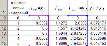
For each series of measurements, it is necessary to calculate using formulas (14)l av and T av and then build dependencyT cf 2 \u003d f (l cf) ... For convenience, we introduce the notation:T cf 2 \u003d y 1, l cf \u003d x 1.
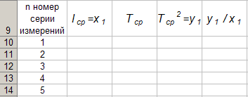
Before proceeding to the indicated calculations, we construct in the programExcel table 3 and prepare the format of table 4, the data of which will be used when constructing the functional dependencey 1 \u003d f (x 1).
In Excel Table 3 is formed as follows.
On Sheet1 of the workbookExcel activate a range of cells cellA 1: A 2, merge them and enter the title of the first column into the resulting merged cell from the keyboard: “n measurement number", Activate the range of cellsB 1: C 1, merge them and enter the common header of the second and third columns into the resulting merged cell from the keyboard: “series 1 ", Activate the cellB 2 and enter from the keyboard the subtitle of the second column of Table 3: “l "After which, we activate cell C2 and enter into it from the keyboard the subtitle of the third column of Table 3:"T ". Let's repeat the indicated actions for the remaining columns of Table 3. As a result of the above actions, we get the format of Table 3.
Now let's fill in the resulting format with the data of table 3, as a result of which we get table 3 in the programExcel.

To build the format of table 4 in the programExcel on Sheet1 of the workbookExcel activate the cellA 9 and enter the header of the first column into it from the keyboard: “n B 9 and enter the second column header into it from the keyboard: “l cf \u003d x 1 ". Similarly, we enter from the keyboard the headers of the third, fourth and fifth columns: “T cf "," T cf 2 \u003d y 1 "and" y 1 / x 1 "in cells C 1, D 1 and E 1 respectively. Next, we activate the cellA 10 and enter the number 1 into it from the keyboard, into the cellA 11 digit 2, activate the range of cellsA 10: A 11 and autocomplete to the cellA 14. As a result of performing the above actions, we get table 4.
Table 4.
We will demonstrate the technology of filling the first row of Table 4 by processing measurements of series 1.
For which we program the first formula in (14), we obtainl Wed and put it in table 4.B 10 and enter from the keyboard the formula "\u003d SUM (B3: B7) * (1/5)".
Then we program the second formula in (14).E 2 and enter the formula "\u003d SUM (C3: C7) * (1/5)" from the keyboard.
We get T av and square it, and then calculate the ratio. To do this, activate the cellD 10 and enter the formula "\u003d C10 ^ 2" from the keyboard, then activate the cellE 10 and enter the formula "\u003d D10 / B10" from the keyboard. After all these actions, the first row of Table 4 takes the form

After repeating these calculations for other series, Table 4 takes the final form
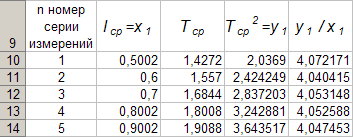
The data in Table 4 allow using the programExcel build a graph of functional dependencey 1 \u003d f (x 1).
To do this, activate the range of cellsD 10: D 14, let's call the Program Function WizardExcel , select the "Scatter" chart type, the first view. Move the mouse cursor to the "Next" button and perform a single click of the left mouse button (LMB). After that, go to the Row tab. To do this, move the mouse cursor in the "Row" tab located in the upper part of the "Chart Wizard" window and perform a single LMB click. Next, place the cursor in the "X Values" field and then move the mouse cursor to the cellB 10, press LMB and without releasing it move the mouse cursor to the cellB 14 and then release LMB. As a result, the formula “\u003d Sheet1! $B $ 10: $ B $ 14 ". Now move the mouse cursor to the "Next" button and perform two LMB clicks in a row, then move the mouse cursor to the "Finish" button and perform a single LMB click. On Sheet1 of the workbookExcel a graph of functional dependence will appeary 1 \u003d f (x 1) ... We activate line 10 and add a new line, after which we enter from the keyboard into the cellsA 10: E 10 digit "0". Next, Move the mouse cursor to any point on the chart and perform a single LMB click. Let's increase the data range of the chart, for which we move the mouse cursor to the border of the range of valuesy 1 and move the marker located in the upper right corner of the border to the cellD 10. Let's do the same with the rangex 1.
Now, move the mouse cursor to any point on the graph and perform a single right-click (RMB). In the context menu that appears, move the mouse cursor to the "Add trend line" command and perform a single LMB click. Figure 4 illustrates the result of these constructions.
Fig 4.
Figure 4 shows that the dependencey 1 \u003d f (x 1) is linear and is described by the equation
y 1 \u003d 4.04 8 x 1 + 0.00 24 (17)
Equation 17 shows that the slopek from equation (10) is equal to:k \u003d 4.0493. If this valuek substituted in formula (12), then we obtain the value of the acceleration of gravity.
Slopek in equation (10) can be calculated from the data in table 4 by the formula
(18)
To do this, activate the cellA 17 and enter the formula “\u003d SUM (E 11: E 15) * (1/5) "
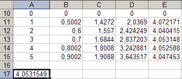
we get k \u003d 4.053, i.e. number close to numberk obtained from the graph shown in Figure 4.
It is obvious that the number obtained by formula (12) using the quantityk from equation (17) will have some error.
To calculate this error, let's return to the data in Tables 3 and 4.
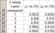
First in the programExcel let's create a new table format 5. Why on Sheet1 of the workbookExcel activate the cellA 19 and enter the header of the first column into it from the keyboard: “n measurement series number ", activate the cellB 19 and enter the second column heading into it from the keyboard: “∆1 according to (15) ". Similarly, enter the headers of the third column from the keyboard: “∆2 to (16) "into cell C 19. Next, activate the cellA 20 and enter the number 1 into it from the keyboard, in the cellA 21 digit 2, activate the range of cellsA 20: A 21 and autocomplete to the cellA 26. As a result of performing the above actions, we get table 5.
Table 5.

When programming formulas (15) and (16), it is necessaryl i and T i , take each series of measurements from Table 3, andl av and T av from the data in Table 4.
To calculate ∆1 for the first series of measurements it is necessary to activate the cellM 3 and enter the formula “\u003d ABS (B3-B $ 11))” into it from the keyboard, then we will autocomplete to the cellM 7. Now into the cellB 20 we will enter from the keyboard the formula "\u003d MAX (M3: M7)".
To calculate ∆2 according to the data of the same series, it is necessary to activate the cellN 3 and enter the formula "\u003d ABS (C3-C $ 11)" into it from the keyboard, after which we will autocomplete to the cellN 7. Now into the cellC 20 we will enter from the keyboard the formula "\u003d MAX (N3: N7)".
As a result, Table 5 takes the form

After performing calculations according to (15) and (16) for data from other series of measurements, Table 5 takes the form
From the data in Table 5, it is obvious that for each series of measurements, the exact length valuesl pendulum and periodT pendulum oscillations are defined as
l \u003d l av ± ∆ 1, T \u003d T av ± ∆ 2 (19)
Moreover, it turns out that ∆1 and ∆ 2 are different for each of the lengths of the pendulum. It follows from formulas (19) that the straight line in Fig. 4 is drawn with an error and in its vicinity there is a so-called scatter of experimental data.
To take into account the scatter of experimental data, let us calculate two more functional dependencies:
(T avg + ∆ 2) 2 \u003d f (l avg + ∆ 1), (20)
(T av - ∆ 2) 2 \u003d f (l av - ∆ 1). (21)
To calculate dependence (20), we introduce new designations:
x 2 \u003d (l cf + ∆ 1), (22)
y 2 \u003d (T avg + ∆ 2) 2, (23)
Before proceeding with the calculations using formulas (22) and (23), we form the format of a new table 6 using the programExcel , according to the previously indicated algorithm, Then we get
Table 6.
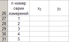
When calculating x 2 and y 2 according to (22) and (23), it is necessary to use the data of Tables 4 and 5. First, we calculatex 2 and the resulting numbers are entered in table 6.
To do this, activate the cellB 27 and enter the formula "\u003d B11 + B20" into it from the keyboard.
Then calculate y 2 for this we activate the cellC 27 and enter the formula "\u003d (C11 + C20) ^ 2" into it from the keyboard.
B 27: C 27 and autocomplete to the cellC 31.
After that, table 6 will be filled with the following data
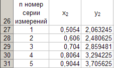
According to table 6 we build a graph of dependencey 2 \u003d y 2 (x 2) (see Fig. 5) according to the previously described technology
Figure 5 shows that the dependencey 2 \u003d y 2 (x 2) is determined by the equation
y 2 \u003d 4.08 86 x 2 - 0.002 3 (24)
We proceed to calculating the functional dependence (21). For this, we introduce two auxiliary formulas
x 3 \u003d l cf - ∆ 1, (25)
y 3 \u003d (T av - ∆ 2) 2. (26)
The calculation according to these formulas is made according to the data of tables 4 and 5, and the results of these calculations are entered in table 7. First, we calculatex 3 ... To do this, activate the cellB 34 and enter the formula "\u003d B11-B20" into it from the keyboard.
Then calculate y 3 for this we activate the cellC 34 and enter the formula "\u003d (C11-C20) ^ 2" into it from the keyboard.
Now let's activate the range of cellsB 34: C 34 and autofill to the cellC 38.
The data in this table are as follows

Functional dependencey 3 = y3 (x3 ) , built according to table 7 is shown in Figure 6.
Figure 6 implies that
y3 = 4,00 7 3 x3 + 0,00 71 (27)
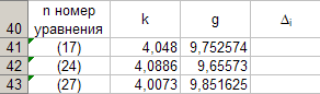
Slope valuesk according to the data of equations (17), (24), (27) we enter into table 8.

We program the formula (12) and calculategcorresponding to each valuek... We enter the obtained valuesg in table 8. To do this, activate the cellC41 and enter the formula "\u003d (4 * PI () ^ 2) / B41" from the keyboard. After that we will autocomplete to the cellC43.
Now we calculate the averageg according to the formula
To do this, activate the cellC45 and enter the formula "\u003d (1/3) * SUM (C41: C43)" from the keyboard.

It turns out to be equal to 9.75331, which we take as the exact value. The error in determining this valueg calculated by the formula
Δ 3 = max | gi gwed| = max | Δ i| (28)
To do this, activate the cellD41 and enter the formula "\u003d ABS (C41-C $ 45)" into it from the keyboard. After that we will autocomplete to the cellD43.

We calculateΔ i and put it in table 8. To do this, activate the cellD45 and enter the formula "\u003d MAX (D41: D43)" from the keyboard.
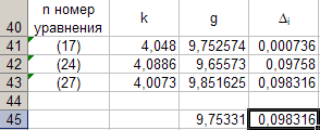
From the data in Table 8 it follows thatΔ 3 \u003d 0.098316. So the accelerationg free fall obtained with this device, as a result of indirect measurements, turned out to be
g \u003d 9.7533 ± 0.0983.
test questions
- What are the elements of the device for studying the oscillations of a mathematical pendulum.
- On the basis of which law of mechanics is the equation of motion of the pendulum compiled.
- Under what constraints an equation is obtained that simulates the movement of a mathematical pendulum.
- What vibrations are called harmonic.
- Give a definition of the amplitude, phase and frequency of oscillations.