Summing specific cells in excel. Selective summation by two criteria

Formulation of the problem

We have a sales table, for example, of the following form:

A task : sum up all orders that manager Grigoriev has implemented for the "Kopeyka" store.

Method 1. SUMIF function

If our task had only one condition (all orders from Grigoriev or all orders to "Kopeyka"), then the task would be solved quite easily using the built-in Excel functionSUMIF browsing the Mathematical category. You can read how to use it. But in our case, there are two conditions, not one, so this method is not suitable ...

Method 2. Column-indicator

Let's add one more column to our table, which will serve as a kind of indicator: if the order was in "Kopeyka" and from Grigoriev, then in the cell of this column there will be a value of 1 otherwise 0. The formula that must be entered into this column is very simple:

\u003d (A2 \u003d "Kopeyka") * (B2 \u003d "Grigoriev")

Boolean equalities in parentheses give TRUE or FALSE, which for Excel equals 1 and 0. So, since we multiply these expressions, 1 will eventually only work if both conditions are true. Now the cost of sales remains to be multiplied by the values \u200b\u200bof the resulting column and sum up the amounts obtained:

Method 3. The magic array formula

If you haven't come across such a wonderful Excel feature as array formulas before, I advise you to read a lot of good things about them beforehand.... Well, in our case, the problem is solved by one formula:

SUM ((A2: A26 \u003d "Penny") * (B2: B26 \u003d "Grigoriev") * D2: D26)

After entering this formula, you must press not Enter, as usual, butCtrl + Shift + Enter - then Excel will perceive it asarray formula and will add the curly braces myself. You do not need to enter parentheses from the keyboard. It is easy to realize that this method (like the previous one) is easily scalable by three, four, etc. conditions without any restrictions.

Method 4. Database function BDSUMM

In category Databases you can find the functionBDSUM (DSUM) , which can also help us solve our problem:

The nuance is that for this function to work, you need to create on the sheet a range of cells containing selection conditions, and then specify this range of the function as an argument:

BDSUMM (A1: D26; D1; F1: G2)

Method 5. Partial Sum Wizard

This is the name of an Excel add-in that helps you create complex formulas for multicriteria summation. You can connect this free add-on through the menuService - Add-ins - Summation Wizard(Tools - Add-Ins - Conditional Sum Wizard)... After that in the menuService the command should appearPartial amount to launch the Summation Wizard:

In the first step Summation wizards you must specify a range with data, i.e. select our entire table. At the second step, you need to select a column for summing and form conditions for selecting values, adding each condition to the list with the buttonAdd condition:

And finally, at the 3rd and 4th steps, we indicate the cell where you want to display the result. And we end up with the following:

It is easy to see that we used something similar to this array formula in Method 3. Only here you can not touch the keyboard at all - long live laziness - the engine of progress!

Did you know, what is a thought experiment, a gedanken experiment?
This is a non-existent practice, an otherworldly experience, the imagination of what is not in reality. Thought experiments are like waking dreams. They give birth to monsters. Unlike a physical experiment, which is an experimental test of hypotheses, a "thought experiment" trickeryly replaces experimental verification with desired, untested in practice conclusions, manipulating logical constructions that actually violate logic itself by using unproved premises as proven ones, that is, by substitution. Thus, the main task of applicants for "thought experiments" is to deceive the listener or reader by replacing a real physical experiment with his "doll" - fictitious reasoning on parole without physical verification itself.
Filling physics with imaginary, "thought experiments" led to the emergence of an absurd surreal, confused and confused picture of the world. A real researcher must distinguish such "wrappers" from real values.

Relativists and positivists argue that the "thought experiment" is a very useful tool for testing theories (also arising in our mind) for consistency. In this they deceive people, since any verification can be carried out only by a source independent of the object of verification. The applicant himself of the hypothesis cannot be a test of his own statement, since the reason for this statement itself is the absence of contradictions in the statement visible to the applicant.

We see this in the example of SRT and GRT, which have turned into a kind of religion that controls science and public opinion... No amount of facts that contradict them can overcome Einstein's formula: "If a fact does not correspond to the theory, change the fact" (In another version "- The fact does not correspond to the theory? - So much the worse for the fact").

The maximum that the "thought experiment" can claim is only the internal consistency of the hypothesis within the applicant's own, often by no means true, logic. This does not test the suitability of practice. The real test can only take place in a valid physical experiment.

An experiment is also an experiment, that it is not a refinement of thought, but a test of thought. A thought that is self-consistent within itself cannot verify itself. This is proven by Kurt Gödel.

FORUM NEWS

Aether knights

10/30/2017 - 06:17: -\u003e - Karim_Khaidarov.
10/19/2017 - 04:24: -\u003e - Karim_Khaidarov.
11.10.2017 - 05:10: -\u003e - Karim_Khaidarov.
05.10.2017 - 11:03:

Function SUMIF is used when it is necessary to sum the range values \u200b\u200bthat meet the specified condition. For example, suppose that in a column of numbers you only want to add up values \u200b\u200bgreater than 5. To do this, you can use the following formula: \u003d SUMIF (B2: B25, "\u003e 5")

This video is part training course Add numbers in Excel 2013.

Advice:

Syntax

SUMIF (range, condition, [sum_range])

Function arguments SUMIF are described below.

Range ... Required argument. The range of cells to be evaluated for compliance. The cells in each range must contain numbers, names, arrays, or number references. Blank cells and cells containing text values \u200b\u200bare skipped. The selected range can contain dates in standard Excel format (see examples below).

Condition ... Required argument. A condition, in the form of a number, expression, cell reference, text, or function, that determines which cells to sum. For example, a condition can be represented as: 32, "\u003e 32", B5, "32", "apples", or TODAY ().

Important: All text conditions and conditions with logical and mathematical signs must be enclosed in double quotes ( " ). If the condition is a number, you do not need to use quotation marks.

Sum_range ... Optional argument. Cells from which values \u200b\u200bare added if they differ from the cells specified as range ... If the argument sum_range omitted, Excel sums the cells specified in the argument range (the same cells to which the condition applies).

In the argument condition wildcards can be used: question mark ( ? ) and an asterisk ( * ). The question mark matches any single character, and the asterisk matches any sequence of characters. If you want to find directly a question mark (or an asterisk), you must put a tilde in front of it ( ~ ).

Notes

SUMIF returns incorrect results when used to match strings longer than 255 characters or when applied to the #VALUE! String.

Argument sum_range may not be the same size as the argument range ... The top-left cell of the argument is used as the starting cell when determining the actual cells to be added sum_range , and then the cells of the part of the range corresponding in size to the argument are summed range ... Example:

Range	Summation range	Actual cells

However, if the arguments range and sum_range Since the SUMIF functions contain a different number of cells, the sheet recalculation may take longer than expected.

Examples of

Example 1

Copy the sample data from the following table and paste it into cell A1 of the new excel worksheet... To display the results of formulas, select them and press F2, and then press Enter. Change the width of the columns as needed to see all the data.

Property value	Commission	Data




Formula	Description	Result
SUMIF (A2: A5; "\u003e 160000"; B2: B5)	The amount of commissions for property worth more than RUB 1,600,000.
SUMIF (A2: A5; "\u003e 160000")	The amount of property worth more than RUB 1,600,000.
SUMIF (A2: A5; 300000; B2: B5)	The amount of commissions for property worth 3,000,000 rubles.
SUMIF (A2: A5; "\u003e" B2: B5)	The amount of commissions for property that exceeds the value in cell C2.

Example 2

Copy the sample data from the table below and paste it into cell A1 of a new Excel sheet. To display the results of formulas, select them and press F2, and then press Enter. In addition, you can adjust the width of the columns according to the data they contain.

	Products	Volume of sales
	Tomatoes
	Celery
	Oranges



Formula	Description	Result
SUMIF (A2: A7, "Fruit", C2: C7)	Sales of all products in the Fruit category.
SUMIF (A2: A7; "Vegetables"; C2: C7)	Sales volume of all products in the category "Vegetables".
SUMIF (B2: B7; "* s"; C2: C7)	Sales volume of all products whose names end with "s" ("Tomatoes" and "Oranges").
SUMIF (A2: A7, "", C2: C7)		additional information You can always ask the Excel Tech Community a question, ask for help in the Answers community, or suggest a new feature or improvement on the website.

Good day!

I will continue my endeavor to describe the variety of functions in Excel and the next one for our consideration. This is another representative of the summation functions, but with its own specific conditions. BDSUMM function in Excel searches for numbers in your table according to the criteria you defined, this is its main property.

In all honesty, I can say that a lot of calculations and calculations can be done without it using various, or SUMPRODUCT, but if you need to make a complex selection using wildcards, then you definitely need to use the hero of our article.

First, let's look at the syntax that uses:

\u003d BDSUMM (your database range; search field; search term)where

When working with function BDSUMM it is worth noting several conditions that you should pay attention to when working:

When working on a whole column filled with data, be sure to insert an empty line under the column headings in the specified range of criteria;
The range of criteria must not overlap with the list;
Although you can place the data to form the range of conditions anywhere on the sheet, you should not place it after the list, since the data that we add to the list will be inserted in the first row after the list, and if there is data in the row, then adding new ones will not work;
You can use any range for conditions that contains at least one heading and at least one of the cells that is located under the heading and contains the condition.

So, the theoretical part, I consider completed, now let's get down to practical application bDSUMM functions in our work, for this we will consider several examples for execution, I did the examples according to the principle, but instead of collecting values \u200b\u200bby criterion, there will be summation:

BDSUMM function with one numerical criterion

So, to begin with, let's look at a simple example with one numerical criterion, for this we select the "Harvest" column and indicate that we need trees with a yield "\u003e \u003d 10". To get the result, we need a formula of this kind (I advise you to use absolute references):

\u003d BDSUMM ($ B $ 6: $ G $ 12; E6; E2: E3),

where, $ B $ 6: $ G $ 12 is the range in which we will summarize, E6 is the column in which we will summarize, and E2: E3 is the range in which we entered the criteria for summing. As a result, the formula found 3 positions for a total of 34.

To obtain a similar result, you can also use the following formulas:

\u003d SUMIF (E7: E12, "\u003e \u003d 10")

\u003d SUMIF (E7: E12, E3)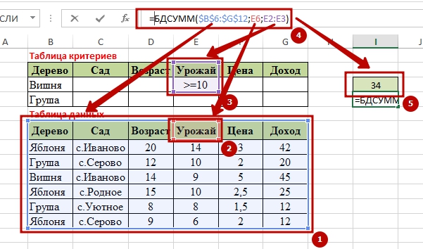

BDSUMM function with one text criterion

Now let's look at how the BDSUMM function behaves with text criteria, in general, everything remains the same in the previous example, except for how the text criterion is indicated, and it is indicated only in this form: \u003d "\u003d s. Serovo" and then you will get the result otherwise the formula will not be able to recognize your criterion. Now we substitute this criterion into the formula and get:

\u003d BDSUMM ($ B $ 6: $ G $ 12; E6; C2: C3), as we see, only the range of the criterion has changed.

To get a similar result, you will need:

\u003d SUMIF (C7: C12, "s.Serovo", E7: E12)

Summation by two criteria over different columns

The example is complicated by the application of two criteria, but we will not apply anything fundamentally new, we will indicate the text criterion "S. Serovo" and the numerical criterion "\u003e \u003d 10", leaving the summation field "Harvest", we will get a change in the formula only for the last argument, as a result ... Our formula will now look like this:

\u003d BDSUMM ($ B $ 6: $ G $ 12; E6; C2: E3), again you see changes only to the address of the criteria range

An alternative option can be obtained using and like this:

\u003d SUMIF (E7: E12; C7: C12; C3; E7: E12; E3)

\u003d SUMIFS (E7: E12; C7: C12; "с.Serovo"; E7: E12; "\u003e \u003d 10")

Summation over one of two conditions in one column

Let's consider another option as applied, but now we will use not a single criterion, but a double one, but for one field. The two criteria must be on different lines. The essence of the formula boils down to the fact that it goes through the same range twice, counting each of the criteria separately. For this example, the formula would look like this:

\u003d BDSUMM ($ B $ 6: $ G $ 12; E6; C2: C4), here we again change the range of the criterion, but not in width, but in height.

Also as a substitute, you can use the sum of the SUMIF function:

\u003d SUMIF (C7: C12; C3; E7: E12) + SUMIF (C7: C12; C4; E7: E12).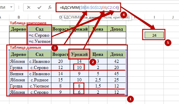

Summation over one of two conditions in two different columns

The fifth application example will be the summation over one of the two conditions in two different columns and the arguments must be placed all in new lines, this will allow them to be summed up in turn. For these purposes, we need a formula:

\u003d BDSUMM ($ B $ 6: $ G $ 12; D6; C2: D4), the principle of forming the formula is preserved, except for the range of criteria, which includes three lines: a title and two criteria.

Summation by two text criteria by two columns

In this example of work, we will consider an almost complete analogue of the previously considered example, when there were two criteria in two columns, but there was a numerical and a text criterion, but here we will consider the summation by two text criteria and by two columns. We use the criteria "\u003d" \u003d s.Ivanovo "" and "\u003d" \u003d Cherry "", which we will indicate in the range of criteria. So our formula will look like this:

\u003d BDSUMM ($ B $ 6: $ G $ 12; D6; B2: C3).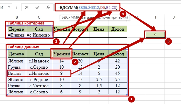

Using the result of a formula to obtain a selection criterion and summation

In this example of the BDSUMM function, I use a formula to determine the selection and summation criterion, in this case we will find which trees generate income for us and to determine the conditional argument we take the average value for the sales of fruits from trees and everything above the average is of interest to us. To determine the average value that will become our TRUE criterion, we create the formula:

\u003d G7\u003e AVERAGE ($ G $ 7: $ G $ 12), do not forget about to fix the range, so that when the formula goes through the values, they do not slide down, but the G7 value should slide over the entire range to determine whether it is "FALSE" or "TRUE".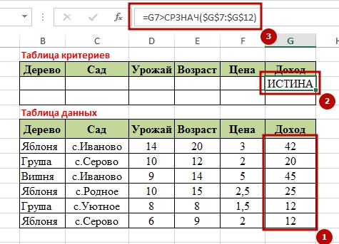

It is also very important that the titles of the headings are not duplicated, have a difference, so I will name the criteria field "Average". And then the formula will start working, it will iterate over the entire range of $ G $ 7: $ G $ 12 for the presence of an average value, and when a positive result is "TRUE", it will sum. The following formula will cope with this work:

\u003d BDSUMM ($ B $ 6: $ G $ 12; G6; $ G $ 2: $ G $ 3)

And if you are very interested in an alternative solution to the question, then try the option with the SUMIF function in this form:

\u003d SUMIF ($ G $ 7: $ G $ 12; "\u003e" & AVERAGE ($ G $ 7: $ G $ 12))

BDSUMM function according to three criteria

In this example, let us calculate the average sales per fruit grown in two villages: “Ivanovo village” and “Uyutnoe village”. I have already described the main idea of \u200b\u200bselection by criteria, so I will not repeat myself, I will simply say that it will be a combination of the previously considered criteria. To get the result, we need it in this form:

\u003d BDSUMM ($ B $ 6: $ G $ 12; G6; $ C $ 2: $ G $ 4)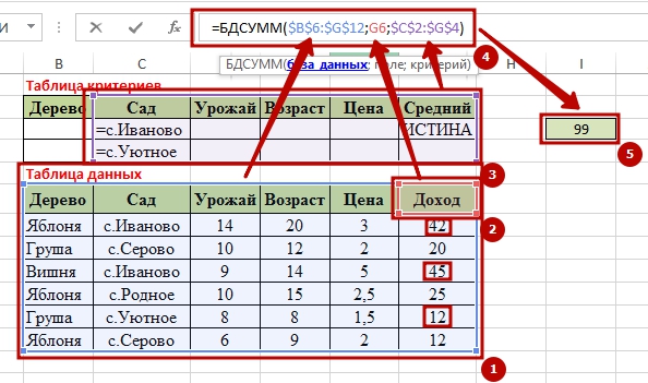

Summation by text criterion, case sensitive

As I mentioned earlier, it can search not only with wildcards, but also case-sensitive, now this is exactly the option. To begin with, we define the condition for the selection of a criterion, if the name "s. IVANOVO" is encountered, in capital letters, then we perform the summation, to determine this criterion we need the formula:

\u003d COUNCIL ("S. IVANOVO"; C7)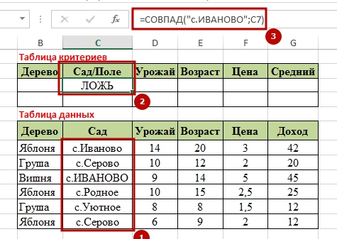

But now we can write a function that will check the range for the presence of the specified criterion and, when the value "TRUE" is received, will perform the summation. In the example, I specifically indicated one time according to the condition, and as you can see, the formula successfully selected all settlements and found the desired one and got the result "9". For this, the formula was used:

\u003d BDSUMM ($ B $ 6: $ G $ 12; D6; $ C $ 2: $ C $ 3)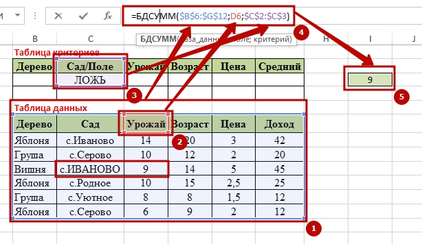

Well, I think that I described the detail in many details, so there will be few questions, but a lot of benefits. If you have any questions, write comments, I look forward to your likes and reviews. You can find out about other functions on my website.