Setting a dash in Microsoft Excel
Excel often has to process text strings in one way or another. It is very difficult to do such operations manually when the number of lines is more than one hundred. For convenience, Excel has a fairly good set of functions for working with a string data set. In this article I will briefly describe the necessary functions for working with strings of the "Text" category and will consider some of them with examples.
Functions of the "Text" category
So, let's look at the basic and useful functions of the "Text" category, the rest can be found on your own.
- BATTEXT (Value) - a function that converts a number to a text type;
- DLSTR (Value) is a helper function, very useful when working with strings. Returns the length of the string, i.e. number of characters contained in the string;
- REPLACE (Old text, Start position, number of characters, new text) - replaces the specified number of characters from a certain position in the old text with a new one;
- SIGNIFICANT (Text) - converts text to number;
- LEVSIMV (String, Number of characters) - a very useful function, it returns the specified number of characters, starting from the first character;
- RIGHT (String, Number of characters) - analog of the function LEVSIMV, with the only difference that characters are returned from the last character of the string;
- TO FIND (text to be searched, text in which we are looking, starting position) - the function returns the position from which the search text begins to appear. The characters are case sensitive. If you need to be case insensitive, use the function SEARCH... Only the position of the first occurrence in the string is returned!
- SUBSTITUTE (text, old text, new text, position) - an interesting function, at first glance it looks like a function REPLACEbut the function SUBSTITUTE can replace all occurrences in the string with a new substring if the "position" argument is omitted;
- PSTR (Text, Start Position, Number of Characters) - the function is similar to LEVSIMV, but is capable of returning characters from the specified position:
- COUPLING (Text1, Text 2 .... Text 30) - the function allows you to connect up to 30 lines. Also, you can use the symbol " & ”, It will look like this“ \u003d ”Text1” & ”Text2” & ”Text3” ”;
These are mostly commonly used functions when working with strings. Now let's look at a couple of examples to demonstrate how some of the functions work.
Example
1
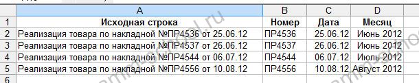
Given a set of lines:
It is necessary to extract dates, invoice numbers from these lines, as well as add a month field to filter lines by month.
Let's extract the invoice numbers into column B. To do this, we will find the so-called key symbol or word. In our example, you can see that each invoice number is preceded by "No.", and the length of the invoice number is 6 characters. Let's use the FIND and PSTR functions. We write the following formula in cell B2:
= PSTR(A2; TO FIND("No."; A2) +1; 6)
Let's analyze the formula. From the line A2 from the position next after the found character "No.", we extract 6 characters of the number.
Now let's extract the date. Everything is simple here. The date is located at the end of the line and is 8 characters long. The formula for C2 is as follows:
= RIGHT(A2; 8)
but the extracted date will be a string, in order to convert it to a date it is necessary after extraction, the text should be converted to a number:
= SIGNIFICANT(RIGHT(A2; 8))
and then, set the display format in the cell, as described in the article "".
And finally, for the convenience of further filtering the rows, we will introduce the month column, which we will get from the date. Just to create a month, we need to discard the day and replace it with "01". Formula for D2:
= SIGNIFICANT(COUPLING("01"; RIGHT(A2; 6))) or \u003d SIGNIFICANT("01"& RIGHT(A2; 6))
Format the cell " MMMM YYYY". Result:
Example 2
In line " An example of working with strings in Excel"it is necessary to replace all spaces with" _ ", also add" MS "before the word" Excel ".
The formula will be as follows:
=SUBSTITUTE(REPLACE(A1; SEARCH("excel"; A1); 0; "MS"); ""; "_")
In order to understand this formula, break it down into three columns. Start with SEARCH, the last one will be SUBSTITUTE.
All. If you have any questions, ask, do not hesitate
The following functions find and return parts of text strings or make large strings from small ones: FIND, SEARCH, RIGHT, LEFT, MID, SUBSTITUTE, REPT, REPLACE, CONCATENATE.
FIND and SEARCH functions
The FIND and SEARCH functions are used to determine the position of one text string in another. Both functions return the character number from which the first occurrence of the search string begins. These two functions work the same way, except that FIND is case-sensitive and SEARCH accepts wildcard characters. Functions have the following syntax:
\u003d FIND (lookup_text; lookup_text; start_position)
\u003d SEARCH (lookup_text; lookup_text; start_position)
Argument search_text specifies the text string to find, and the argument viewed_text - the text in which the search is performed. Any of these arguments can be a character string, enclosed in double quotes, or a cell reference. Optional argument start_position specifies the position in the viewed text from which the search begins. Argument start_position should be used when lookup_text contains multiple occurrences of the search text. If this argument is omitted, Excel returns the position of the first occurrence.
These functions return an error value when search_text is not contained in the text being viewed, or start_position is less than or equal to zero, or start_position exceeds the number of characters in the text being viewed, or start_position greater than the position of the last occurrence of the search text.
For example, to determine the position of the letter "g" in the line "Garage doors", you must use the formula:
FIND ("f"; "Garage doors")
This formula returns 5.
If you do not know the exact character sequence of the text you are looking for, you can use the SEARCH function and include search_text wildcard characters: question mark (?) and asterisk (*). A question mark matches a single randomly typed character, and an asterisk replaces any sequence of characters at the specified position. For example, to find the position of the names Anatoly, Alexey, Akaki in the text located in cell A1, you need to use the formula:
SEARCH ("A * d"; A1)
Functions RIGHT and LEFT
The RIGHT function returns the rightmost characters in the argument string, while the LEFT function returns the first (left) characters. Syntax:
\u003d RIGHT (text, num_chars)
\u003d LEFT (text, num_chars)
Argument characters specifies the number of characters to extract from the argument text ... These functions are whitespace-aware and therefore if the argument text contains spaces at the beginning or end of a line, use the TRIM function in function arguments.
Argument number of characters must be greater than or equal to zero. If this argument is omitted, Excel considers it to be 1. If characters more characters in the argument text , then the entire argument is returned.
PSTR function
The MID function returns a specified number of characters from a string of text, starting at a specified position. This function has the following syntax:
\u003d MID (text; start_position; number of characters)
Argument text is a text string containing the characters to be extracted, start_position is the position of the first character to be extracted from the text (relative to the beginning of the line), and characters is the number of characters to extract.
REPLACE and SUBSTITUTE functions
These two functions replace characters in text. The REPLACE function replaces part of a text string with another text string and has the syntax:
\u003d REPLACE (old_text; start_position; number of characters; new_text)
Argument old_text is a text string to replace characters with. The next two arguments specify the characters to be replaced (relative to the beginning of the line). Argument new_text specifies the text string to insert.
For example, cell A2 contains the text "Vasya Ivanov". To put the same text in cell A3, replacing the name, you need to insert the following function into cell A3:
REPLACE (A2; 1; 5; "Petya")
In the SUBSTITUTE function, the starting position and the number of characters to be replaced are not specified, but the replacement text is explicitly specified. The SUBSTITUTE function has the following syntax:
\u003d SUBSTITUTE (text; old_text; new_text; entry_number)
Argument entry_number is optional. It instructs Excel to replace only the given occurrence of the string old_text .
For example, cell A1 contains the text "Zero less than eight". It is necessary to replace the word "zero" with "zero".
SUBSTITUTE (A1; "o"; "y"; 1)
The number 1 in this formula indicates that only the first "o" in the row of cell A1 needs to be changed. If the argument entry_number omitted, Excel replaces all occurrences of the string old_text per line new_text .
REPEAT function
The REPT function allows you to fill a cell with a string of characters repeated a specified number of times. Syntax:
\u003d REPEAT (text, repetitions)
Argument text is a multiplied string of characters, enclosed in quotes. Argument repetitions indicates how many times to repeat the text. If the argument repetitions is 0, the REPEAT function leaves the cell empty, and if it is not an integer, this function discards the decimal places.
CONCATENATE function
The CONCATENATE function is the equivalent of a text statement & and is used to concatenate strings. Syntax:
\u003d CONCATENATE (text1, text2, ...)
You can use up to 30 arguments in a function.
For example, cell A5 contains the text "first half of the year", the following formula returns the text "Total for the first half of the year":
CONCATENATE ("Total for"; A5)
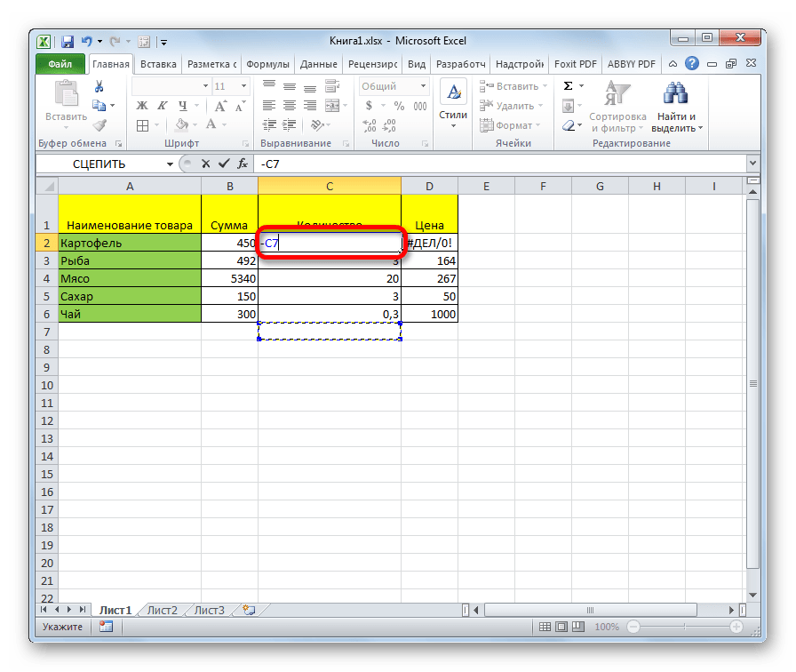
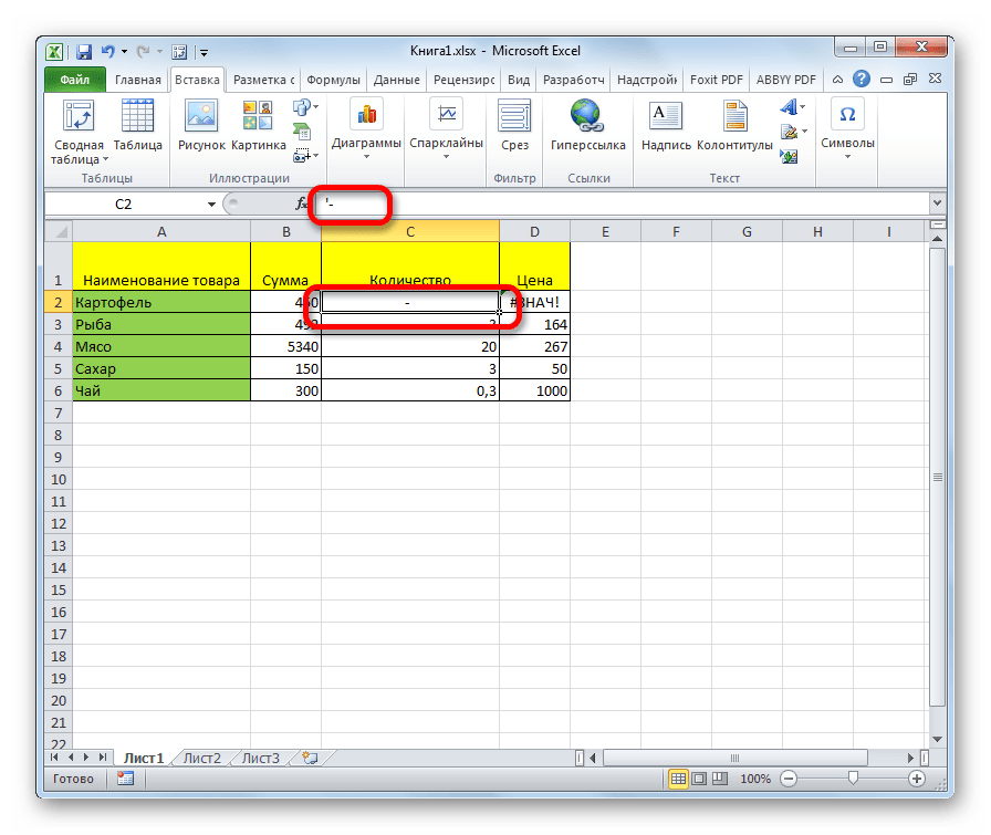
Many Excel users experience considerable difficulty when trying to put a dash on a worksheet. The fact is that the program understands a dash as a minus sign, and immediately converts the values \u200b\u200bin the cell into a formula. Therefore, this issue is quite urgent. Let's see how to put a dash in Excel.
Often, when filling out various documents, reports, declarations, you need to indicate that the cell corresponding to a specific indicator does not contain values. For these purposes, it is customary to use a dash. For the Excel program, this possibility exists, but it is rather problematic to implement it for an unprepared user, since the dash is immediately converted into a formula. To avoid this transformation, you need to perform certain actions.
Method 1: formatting the range
The most famous way to put a dash in a cell is to give it a text format. However, this option does not always help.

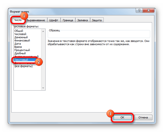
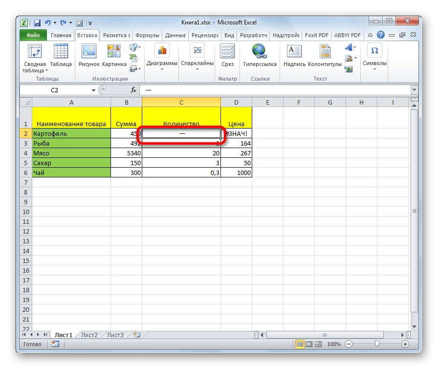
After that, the selected cell will be assigned the property text format... All values \u200b\u200bentered into it will be perceived not as objects for calculations, but as plain text. Now in this area you can enter the symbol "-" from the keyboard and it will be displayed exactly as a dash, and will not be perceived by the program as a minus sign.

There is one more option for reformatting a cell to a text view. To do this, being in the tab "The main", you need to click on the drop-down list of data formats, which is located on the ribbon in the toolbox "Number"... A list of available formatting types opens. In this list, you just need to select the item "Text".

Method 2: Pressing the Enter Button
But this method does not work in all cases. Often, even after this procedure, when you enter the character "-" instead of the character needed by the user, all the same references to other ranges appear. In addition, it is not always convenient, especially if cells with dashes in the table alternate with cells filled with data. Firstly, in this case, you will have to format each of them separately, and secondly, the cells of this table will have a different format, which is also not always acceptable. But you can do it in another way.

This method is good for its simplicity and the fact that it works with any kind of formatting. But, at the same time, when using it, you need to be careful about editing the contents of the cell, since due to one wrong action, a formula may appear again instead of a dash.
Method 3: insert a symbol
Another way to write a dash in Excel is to insert a symbol.


After that, the dash will be reflected in the selected cell.
There is another option for this method. Being in the window "Symbol", go to the tab "Special characters"... In the list that opens, select the item Em dash... Click on the button "Paste"... The result will be the same as in the previous version.

This method is good in that you will not need to be afraid of the wrong movement of the mouse. The symbol will still not change to a formula. In addition, visually a dash delivered in this way looks better than a short character typed from the keyboard. The main disadvantage of this option is the need to perform several manipulations at once, which entails temporary losses.
Method 4: add an extra character
In addition, there is another way to put a dash. True, visually, this option will not be acceptable for all users, since it assumes the presence in the cell, in addition to the "-" sign, one more symbol.

There are a number of ways to set a dash in a cell, the choice between which the user can make according to the purpose of using a particular document. Most people try to change the format of the cells at the first unsuccessful attempt to put the desired character. Unfortunately, this does not always work. Fortunately, there are other options for accomplishing this task: go to another line using the button Enter, the use of symbols through the button on the ribbon, the use of an additional sign "’ ". Each of these methods has its own advantages and disadvantages, which were described above. There is no universal option that would be most suitable for installing a dash in Excel in all possible situations.