Excel how to summarize certain criteria. Finance in Excel
One day life circumstances force you to master new software tools for solving everyday or office tasks. To do it manually is long and inconvenient, besides, the probability of making a mistake increases. Therefore, let's look at how SUMIF works in Excel and show examples of use.
Function syntax and working principle
The possibilities of addition are known to every user who has launched Excel at least once. SUMIF is a logical continuation of the basic SUM, the difference of which is summation by condition.
The syntax for SUMIF is as follows:
\u003d SUMIF (range, criterion, [summation range])where:
- range - a list of values \u200b\u200bto which the restriction will be applied;
- criterion - a specific condition;
- summation range - a list of values \u200b\u200bthat will be summed.
So, we have a function with three components. It is worth noting that the last argument can be omitted - SUMIF is capable of working without a summation range.
Examples of using
Let's consider all possible situations of using the function of the same name.
General form
Let's look at a simple example to illustrate the benefits of using SUMIF.
There is a table that contains the serial number, type of product, name, unit price and number of pieces in stock.
Let's say we need to figure out how many items are in stock. Everything is simple here - we use the SUM and specify the desired interval. But what if you are interested in the number of items of clothing? This is where SUMIF comes to the rescue. The function will look like this:
\u003d SUMIF (C3: C12; "clothes"; F3: F12)where:
- C3: C12 - type of clothing;
- “Clothes” is a criterion;
- F3: F12 - summation interval.

As a result, we got 180. The function worked through all the conditions we specified and produced the correct result. You can also repeat similar manipulations for other types of goods by changing the criterion "clothes" to some other one.
With multiple conditions
We need this option in cases where, in addition to clothes, we are also interested in the cost of a unit of goods. Those. except for one condition, you can use two or more. In this case, we need to register a slightly modified function - SUMIF. The suffix MH means many conditions (at least 2), which we will now demonstrate to you. The function will look like:
\u003d SUMIFS (F3: F12; C3: C12; "clothes"; E3: E12; 50)where:
- F3: F12 - summation range;
- "Clothes" and 50 - criteria;
- C3: C12 and E3: E12 are the ranges of product types and unit values, respectively.
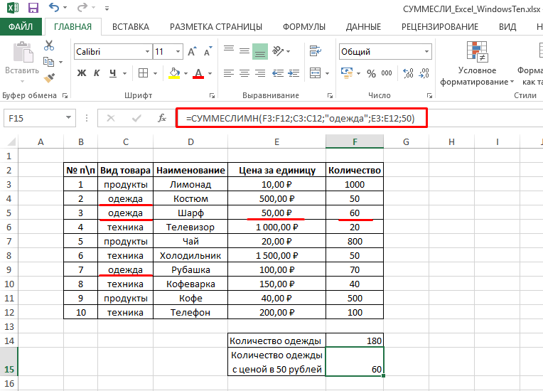
Attention! In the SUMIFS function, the sum range argument appears at the beginning of the formula. Be careful!
With dynamic condition
There are situations when we forgot to add one of the products to the table and needs to be added. The situation is saved by the fact that the SUMIF and SUMIFS functions automatically adjust to changes in the data in the table and instantly update the total value.
To insert a new line, you need to right-click on the cell of interest and select "Insert" - "Line". 
Then just enter the new data or copy it from another location. The final value will change accordingly. Similar transformations occur when editing or deleting lines. 
This is where I end. You have seen basic examples of using the SUMIF function in Excel. If you have any recommendations or questions - you are welcome in the comments.
SUMIF function. The first of three Excel whales. I'm starting to review the main tools of our favorite Microsoft program. And of course, first I want to talk about my most frequently used function ("formula"). More precisely, the SUMIF function. If you have no idea what it is and how to use it - I envy you! It was a real discovery for me.
Did you have to summarize data on employees or customers from a large table, choose how much revenue was for a particular item? You filtered by last name / position, and then entered numbers manually into individual cells? Maybe they counted on a calculator? And if there are more than a thousand lines? How to calculate quickly?
This is where SUMIF comes in handy!
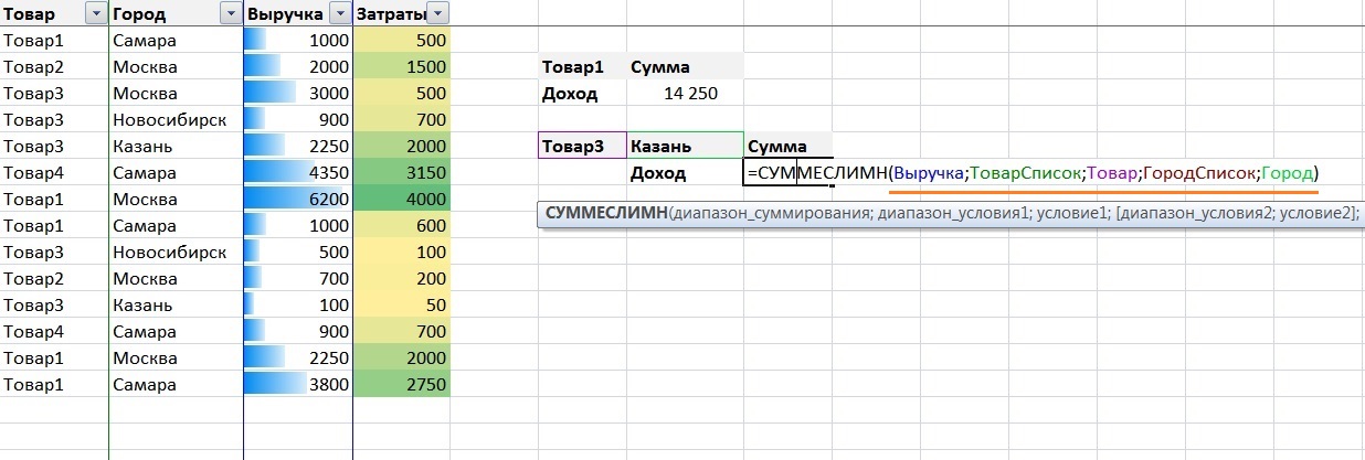
Task1... There are statistics on goods, cities and what indicators were achieved for these items. It is necessary to calculate: "for how much was sold the item Commodity1? "
How does the SUMIF function in Excel work? Counting sum by value
Before proceeding to the solution of the 1st problem, let's analyze what the SUMIF function consists of:
- Range. The range that contains the search terms. Required. For the 1st task, the Product column.
- Criterion. Can be filled with number (85), expression ("\u003e 85"), cell reference (B1), function (today ()). Defines the condition by which (!) Are summed up. All text conditions are enclosed in quotation marks ( « ) "\u003e 85". Required. For the 1st task, column \u003d Product1
- Sum_range. Cells to add if they are different from cells in Range. For the 1st task, the Revenue column.
So, let's write the formula, having previously entered the condition argument into cell F3
Don't forget to check;) Did it count? Right? Fine!
How does the SUMIFS function in Excel work? Calculating the sum by values
Those. the selection must be performed according to two parameters. For this, the SUMIF function is used for several conditions - SUMIF, where the order of writing and the number of arguments are slightly changed.
Now we will look at another very frequently used Excel function - SUMIF.
Let's look at one example of using the SUMIF function. Suppose that in the source data we have a table for orders in different cities. Each line displays the number of orders in a specific city on a specific date (which date we are not interested in in this task).
Our task is to calculate the sum of all orders by city for the entire period. This task can be easily handled excel function - SUMIF. As the name implies, this function sumsiterates values if a they meet certain criteria.
SUMIF (range, criterion, sum_range)
In our example, we need to fill in the second table on the right - the column for the amount of orders by city. As you can see from the syntax of the SUMIF function, we need three arguments.
range - this is the comparison range, that is, the array in which the criteria will be compared. In our example, this is A5: A504 so that when stretching the formula our range does not shift, we will make it absolute by putting the $ sign. We get -$ A $ 5: $ A $ 504
criterion Is an argument, which can be specified as a number, expression, text, etc., which determines which cells to sum up. In our example, the criteria are cities.
sum_range - this is the range that needs to be summed up if the criteria match. In our example, this is the range: B5: B504 , which we will also turn into absolute $ B $ 5 for convenience: $ B $ 504
An example of using the SUMIF function
To solve the problem with this example, write the following formula in cell F5:
SUMIF ($ A $ 5: $ A $ 504; E5; $ B $ 5: $ B $ 504)
The logic of the SUMIF function is as follows: in the range $ A $ 5: $ A $ 504 looking for criterion E5 (St. Petersburg), if St. Petersburg is located, then the number of orders from this line is summed up, that is, from the range $ B $ 5: $ B $ 504

This is a simple example of using the SUMIF function, in the future we will consider this function in more detail with examples of using this function.
We hope this article was helpful to you. If you have any questions, be sure to ask them.
We will be grateful if you click +1 and / or I like at the bottom of this article or share with your friends using the buttons below.
Thanks for attention.
Function SUMis probably the most commonly used. But sometimes you need more flexibility than it can provide. Function SUMIF useful when calculating notional amounts. For example, you might want to get the sum of only negative values \u200b\u200bin a range of cells. This article demonstrates how to use the function SUMIF for conditional summation using one criterion.
The formulas are based on the table shown in Fig. 118.1 and configured to track accounts. Column F contains a formula that subtracts the date in column E from the date in column D. A negative number in column F means that the payment is late. The sheet uses named ranges corresponding to the labels on line 1.
Figure: 118.1. A negative value in column F indicates a late payment Summing only negative values
The following formula returns the sum of negative values \u200b\u200bin column F. In other words, it returns the total number of days overdue for all accounts (for the table in Figure 118.1, the formula will return -63):
\u003d SUMIF (Difference; ".
Function SUMIF can take three arguments. Since you are omitting the third argument, the second argument (") refers to range values Difference.
Sum values \u200b\u200bbased on different ranges
The following formula returns the sum of the overdue invoice volumes (in column C): \u003d SUMIF (Difference; ". This formula uses values \u200b\u200bin the range Differenceto determine if the corresponding values \u200b\u200bof the range contribute to the sum Amount.
Sum values \u200b\u200bbased on text comparison
The following formula returns the total invoice amount for the Oregon office: \u003d SUMIF (Office; "\u003d Oregon"; Amount).
The equals sign is optional. The following formula gives the same result:
To sum the bills for all offices except Oregon, use the following formula:
\u003d SUMIF (Office; "Oregon"; Amount).
Sum values \u200b\u200bbased on date comparisons
The following formula returns the total for invoices due on or after May 10, 2010:
\u003d SUMIF (Date; "\u003e \u003d" & DATE (2010: 5; 10); Amount).
Note that the second argument to the function SUMIF is an expression. The expression uses the function THE DATEwhich returns the date. In addition, the quoted comparison operator is concatenated (using the & ) with the result of the function THE DATE.
The following formula returns the total amount of invoices that are not due (including today's invoices):
\u003d SUMIF (Date; "\u003e \u003d" & TODAY (); Sum).
Acute stomatitis in adults is a disease of viral etiology that occurs in both adults and children. IN recent times Acute herpetic stomatitis is considered as a manifestation of primary herpes infection with the herpes simplex virus in the oral cavity. The incubation period of the disease lasts 1-4 days. The prodromal period is characterized by an increase in the submandibular (in severe cases, cervical) lymph nodes. The body temperature rises to 37-41 ° C, weakness, pallor of the skin, headache and other symptoms are noted.