Excel pivot table totals by row. Display of the '' top ten '' data. Detailed data display
One of the more annoying things about pivot tables is that the grand total, where the data is summed up, is always at the bottom of the table, which means you have to scroll through the entire table just to see the numbers. Let's move the grand total to the top where it's easier to find.
While pivot tables are a great tool for summarizing data and highlighting meaningful information, they do not have a built-in feature to move the grand total to the top where it is easy to find. Before we describe a very general way to move the grand total to the top, let's first see how you can do this using the GETPIVOTDATA function, which is specifically for retrieving data from a pivot table.
This function can be used like this: \u003d GETPIVOTDATA ("Sum of Amount"; $ B $ 5), in the Russian version of Excel \u003d GET.DATA.PERSONAL.TABLE ("Sum by field"; $ B $ 5) or like this: \u003d GETPIVOTOATA (" Amount "; $ B $ 5), in the Russian version of Excel GET.DATA.COMPLETE.TABLES (" Amount "; $ In $ 5).
Both functions will highlight the data you want and track the grand total as you move it up, down, left, or right. We used the cell address $ B $ 5, but if you specify any cell within the pivot table, you will always get the total.
The first function uses the Sum of Amount field, and the second uses the Amount field. If there is an Amount field in the Data area of \u200b\u200bthe PivotTable, you must name the field Amount. If, however, the Amount field is used multiple times in the Data area, you must specify the name you assigned to it, or the default name (Figure 4.5).
To change these fields, you need to double-click them. This can be confusing if you don't fully understand pivot tables yet. Fortunately, in Excel 2002 and later, the process is much easier because you can place arguments in a cell and apply the correct function syntax using the mouse. In any cell, enter \u003d (equal sign) and click the cell that contains the grand total. Excel will automatically insert the required arguments.
Unfortunately, if you use the Function Wizard or first type \u003d GET.PIVOTDATA () (\u003d GETPIVOTDATA ()) and then click on the cell that contains the grand total, Excel will create a mess by trying to put into this cell one more function GETPIVOTDATA.
Probably the easiest and less confusing way to get the grand total is to use the function \u003d МАХ (PivGTCol), in the Russian version of Excel \u003d MAKC (PivGTCol), where the column containing the grand total is named PivGTCol.
In addition, you can use the LARGE and SMALL functions to retrieve a collection of numbers from a pivot table based on how large they are. For example, the following formula selects the second largest number from the pivot table: \u003d LARGE (PivGTCol; 2), in the Russian version of Excel \u003d LARGE (PivGTCol; 2).
You can add multiple rows immediately above the pivot table and place these formulas there so that you can see this type of information immediately without having to scroll to the bottom of the pivot table.
There is a special toolbar for working with pivot tables PivotTable , which allows you to quickly perform basic operations related to editing and formatting pivot tables.
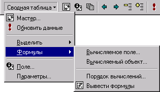 Drop-down menu PivotTable
the toolbar contains operations that are carried out on the panel itself and some other commands. For example, using the submenu Formulas
you can create a calculated field and set the order of calculations.
Drop-down menu PivotTable
the toolbar contains operations that are carried out on the panel itself and some other commands. For example, using the submenu Formulas
you can create a calculated field and set the order of calculations.
Team Options allows you to define the name of the pivot table, display and formatting options, as well as configure external data options if the table is being built on an external data source
Data extraction.
There are two modes of highlighting data in a pivot table: You can select parts of the table or use normal selection. By default, the selection mode is enabled for entire parts of the pivot table. In this mode, by clicking on the field header, you will select it together with the field elements, and when you click on the field element, the data corresponding to this element will also be selected. Moreover, highlighting parts of the pivot table, you highlight both the table headers and the data itself. You can select only headers or only data by selecting the appropriate tool in the toolbar PivotTable :
 You can also set the way to select parts of the pivot table using the command Select
dropdown menu PivotTable
on the toolbar. Here you can select the entire table as a whole by selecting the command Entire Table
... To switch to the normal selection mode (i.e. select not parts, but cells of the table), press the button
in the same menu. To keep the formats of its regions after updating and changing the structure of the pivot table, the button Enable Selection
must be pressed.
You can also set the way to select parts of the pivot table using the command Select
dropdown menu PivotTable
on the toolbar. Here you can select the entire table as a whole by selecting the command Entire Table
... To switch to the normal selection mode (i.e. select not parts, but cells of the table), press the button
in the same menu. To keep the formats of its regions after updating and changing the structure of the pivot table, the button Enable Selection
must be pressed.
Fields, field items, and totals can be removed from the PivotTable. To do this, select the part of the table to be deleted (button Enable Selection must be pressed) and select the command Delete from the context menu.
Updating the original data.If you changed the data in the original tables, you need to update the PivotTable based on that data. To do this, click on the button toolbars PivotTable or choose a command Refresh Data from the dropdown menu PivotTable ... The data is also updated if you added rows (or columns in the case of ranges consolidation) inside original ranges.
If rows or columns have been added to original ranges, you need to call the pivot table wizard by clicking on the button PivotTable Wizard on the toolbar. Returning to the second step of the wizard, you can override the original ranges.
General and subtotals. By choosing the command Options
from the dropdown menu PivotTable
, You can specify whether the pivot table needs a total by rows and / or columns. If the pivot table has a page field, and some of the values \u200b\u200bof this field are hidden, here you can also clarify whether the totals include data corresponding to the hidden values \u200b\u200bof the page fields. If the checkbox Subtotal hidden page items (include hidden values)
disabled, when viewing a pivot table that matches all values \u200b\u200bof a page field, hidden values \u200b\u200bwill not be included in the grand totals.
By choosing the command Options
from the dropdown menu PivotTable
, You can specify whether the pivot table needs a total by rows and / or columns. If the pivot table has a page field, and some of the values \u200b\u200bof this field are hidden, here you can also clarify whether the totals include data corresponding to the hidden values \u200b\u200bof the page fields. If the checkbox Subtotal hidden page items (include hidden values)
disabled, when viewing a pivot table that matches all values \u200b\u200bof a page field, hidden values \u200b\u200bwill not be included in the grand totals.
If a pivot table has multiple column-oriented fields or multiple page-oriented fields, the user can define subtotals for each such field.

 To define subtotals for a field, just double-click on it or select the icon PivotTable Field
on the toolbar. Subtotals for a field can be selected
To define subtotals for a field, just double-click on it or select the icon PivotTable Field
on the toolbar. Subtotals for a field can be selected
- automatic - the amount will be calculated for each element of the field. Automatic totals can be selected only for the external field (in our example, this field year);
- calculated using a standard function selected from the list (you can select several such totals for both external and internal fields);
- abandon intermediate results altogether.
Data grouping.
 It may happen that you need totals not for all elements of the field, but for some groups of data within the field (for example, the elements of the field are the names of months, and the totals must be summed up by quarters). In this case, the field elements can be grouped by selecting them and clicking on the icon Group
on the toolbar. You will have one more field, the elements of which will be the group headers. Moreover, each ungrouped element forms an independent group, the name of which coincides with the name of the element. In the above example, there is one column field containing four elements: january, february, march and april... Three elements ( january, february, march) have been grouped. Element april was not included in the group. As a result, another field appeared month2containing two elements: Group1 and april... Field month still contains the names of the months: january, february, march and april... Field month2 is an external field, i.e. groups the inner field month... You can define subtotals for a new field and the required totals will be calculated for each data group. To ungroup the elements of the field, just select the required group and click on the icon Ungroup
on the toolbar. When there are no grouped items left, the additional outer margin will disappear.
It may happen that you need totals not for all elements of the field, but for some groups of data within the field (for example, the elements of the field are the names of months, and the totals must be summed up by quarters). In this case, the field elements can be grouped by selecting them and clicking on the icon Group
on the toolbar. You will have one more field, the elements of which will be the group headers. Moreover, each ungrouped element forms an independent group, the name of which coincides with the name of the element. In the above example, there is one column field containing four elements: january, february, march and april... Three elements ( january, february, march) have been grouped. Element april was not included in the group. As a result, another field appeared month2containing two elements: Group1 and april... Field month still contains the names of the months: january, february, march and april... Field month2 is an external field, i.e. groups the inner field month... You can define subtotals for a new field and the required totals will be calculated for each data group. To ungroup the elements of the field, just select the required group and click on the icon Ungroup
on the toolbar. When there are no grouped items left, the additional outer margin will disappear.
Calculated fields and field members.
 Usually the table structure is created from the field headers of the original list in the case of a single data range or from objects Line, Column, Value, Pageif there are several ranges. To analyze the data contained in the source tables, the available fields are often insufficient. For example, a pivot table has two data fields: quantity and sum, and you need to determine the average price of the product, which is determined as the quotient of these two fields. In this case, you need to create your own calculated field
- A PivotTable field that uses a user-defined formula that allows you to perform calculations based on the values \u200b\u200bof other fields in the PivotTable. To do this, it is enough to sequentially select the commands Formulas
, Calculated Field
from the dropdown menu PivotTable
... Using the fields that you can select from the list, you can create your own formula for the calculated field. Using the PivotTable Wizard, you can place the new field in the desired area of \u200b\u200bthe PivotTable.
Usually the table structure is created from the field headers of the original list in the case of a single data range or from objects Line, Column, Value, Pageif there are several ranges. To analyze the data contained in the source tables, the available fields are often insufficient. For example, a pivot table has two data fields: quantity and sum, and you need to determine the average price of the product, which is determined as the quotient of these two fields. In this case, you need to create your own calculated field
- A PivotTable field that uses a user-defined formula that allows you to perform calculations based on the values \u200b\u200bof other fields in the PivotTable. To do this, it is enough to sequentially select the commands Formulas
, Calculated Field
from the dropdown menu PivotTable
... Using the fields that you can select from the list, you can create your own formula for the calculated field. Using the PivotTable Wizard, you can place the new field in the desired area of \u200b\u200bthe PivotTable.

 Sometimes reports require not only additional fields, but also field elements. This happens in cases where you need a field that somehow analyzes the data of the existing field elements. For example, a row field or a column field contains elements quantity and sum, and you need to determine the average price of the product, which is determined as the quotient of these two elements. In such cases, you should not create a calculated field, but calculated item
- a PivotTable field element that uses a user-defined formula that allows calculations to be performed based on the values \u200b\u200bof other PivotTable field elements. To create a calculated item, you must select a field or a field item to which a new object will be added and sequentially select the commands Formulas
, Calculated Item
from the dropdown menu PivotTable
... After that, you should specify the name of the new element and set the formula by which it should be calculated. Formulas that calculate additional items use the names of existing PivotTable field items. If multiple fields have elements with the same name, you must insert the field name before the element name. The new item will be added to the field that you selected (or whose item you selected) before creating the calculated object.
Sometimes reports require not only additional fields, but also field elements. This happens in cases where you need a field that somehow analyzes the data of the existing field elements. For example, a row field or a column field contains elements quantity and sum, and you need to determine the average price of the product, which is determined as the quotient of these two elements. In such cases, you should not create a calculated field, but calculated item
- a PivotTable field element that uses a user-defined formula that allows calculations to be performed based on the values \u200b\u200bof other PivotTable field elements. To create a calculated item, you must select a field or a field item to which a new object will be added and sequentially select the commands Formulas
, Calculated Item
from the dropdown menu PivotTable
... After that, you should specify the name of the new element and set the formula by which it should be calculated. Formulas that calculate additional items use the names of existing PivotTable field items. If multiple fields have elements with the same name, you must insert the field name before the element name. The new item will be added to the field that you selected (or whose item you selected) before creating the calculated object.
To supplement Excel with data processing tools (add-ins Report manager and Finding a solution ), in the dialog Add-ons menu Service check the appropriate radio button and click OK (Fig. 1).
If you are prompted that the selected add-in cannot be found, it is most likely not installed. In this case, install the add-in from the installation diskette.
Fig. 1. Dialog window Add-ons.
Drawing up final reports
The purpose of the assignment: learn to draw up subtotals.
Let's perform, for example, the analysis of values \u200b\u200bfor the table containing data on the purchase of printers and scanners by the enterprise for its departments (Table. 1). This problem can be solved by using ordinary formulas, but using the function of automatic calculation of totals can significantly simplify its implementation.
Table 1
|
Product |
Name |
Price |
Number- in |
Amount |
|
|
Matrix | |||||
|
Matrix | |||||
|
Matrix | |||||
|
Jet |
Epson Stylus 1520 | ||||
|
Jet |
Epson Stylus 3000 | ||||
|
Jet |
Epson Stylus 1500 | ||||
|
Jet |
Epson Stylus Photo 700 | ||||
|
Laser |
HP Laser Jet 4000 | ||||
|
Laser |
HP Laser Jet 5000 | ||||
|
Laser |
HP Laser Jet Color 8500 | ||||
|
Sheet |
Paragon Page 630 | ||||
|
Sheet |
Paragon Page Easy | ||||
|
Tablet |
Paragon 800IIEP | ||||
|
Tablet |
ScanExpress 6000 SP | ||||
|
Tablet |
Paragon 1200 SP | ||||
|
Tablet |
ScanExpress A3 P |
We will find the amounts spent on the purchase separately for all printers and separately for all scanners using the automatic calculation of totals. For this:
Sort the table data by product type first, if it has not already been sorted. As the second sorting criterion, you can set, for example, Name;
Select a table or at least one table cell;
On the menu Data select team Outcome . A dialog box will open Subtotals (Fig. 2.).

Dropdown With every change in select the column heading for which you want to calculate intermediate totals after each data change in the worksheet. (in your case, you should select the element Product).In order for the data to be summed up when determining the totals, from the list field Operation select function Amount. In this dialog box, you must also specify the column whose cells are used to calculate totals. In our case, in order to sum up the indicators of the quantity of goods and the amounts spent on the purchase, in the field Add totals by check the boxes next to the lines Qty and Amount.
As a result of executing the function, the table will be supplemented with rows, which will display the totals for each group separately (Fig. 3). The last row inserted into the table contains information about the grand total.

Fig. 3. The table is an example of using the automatic totals function.
For the data of each column group selected in the dialog Subtotals , the following functions can be performed:
|
Function |
Appointment |
|
Adds all values \u200b\u200band gives a grand total |
|
|
Number of values |
Determines the number of elements in a group |
|
Determines the arithmetic mean of a group |
|
|
Maximum |
Determines the largest value in the group and the largest value in the entire column |
|
Determines the smallest value for each group and for the entire column |
|
|
Composition |
Determines the product of all values \u200b\u200bin the group and the product of the entire column |
|
Number of numbers |
Determines the number of cells containing numeric values \u200b\u200bin a group and the total number of cells with numeric values \u200b\u200bfor all column groups |
|
Unbiased deviation |
Determines the value of the standard deviation for a population if the data is sampled |
|
Offset deviation |
Specifies the standard deviation of a population if the data composes a population |
|
Unbiased variance |
Determines the variance value if the data is sampled |
|
Displaced variance |
Specifies the variance value for a population if the data forms a population |
When calculating the totals, the table was structured - you can see this by looking at the screen. With structure levels, you can provide better visual control of your data. To display only the summary data on the screen, click on the button for the second level of the structure, as a result of which the data of the third level (individual values) will be hidden (Fig. 4, 5). To display the individual values \u200b\u200bagain, you must click on the button for the third level 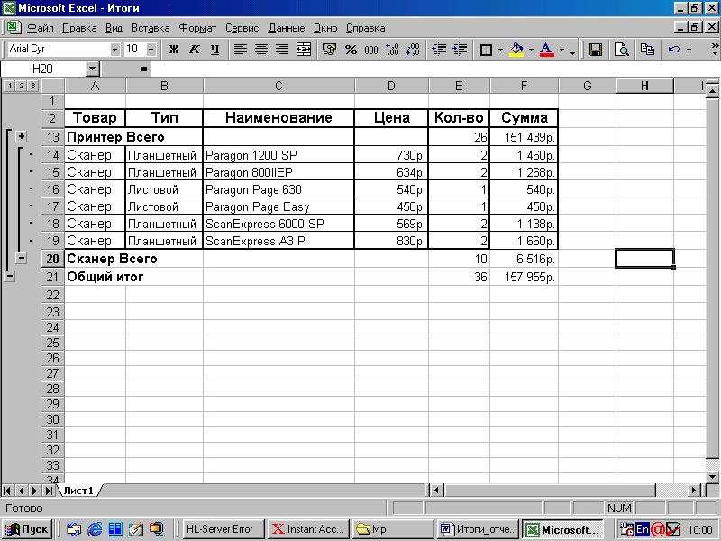
Fig. 4. Option to display the summary data (the third level is hidden).
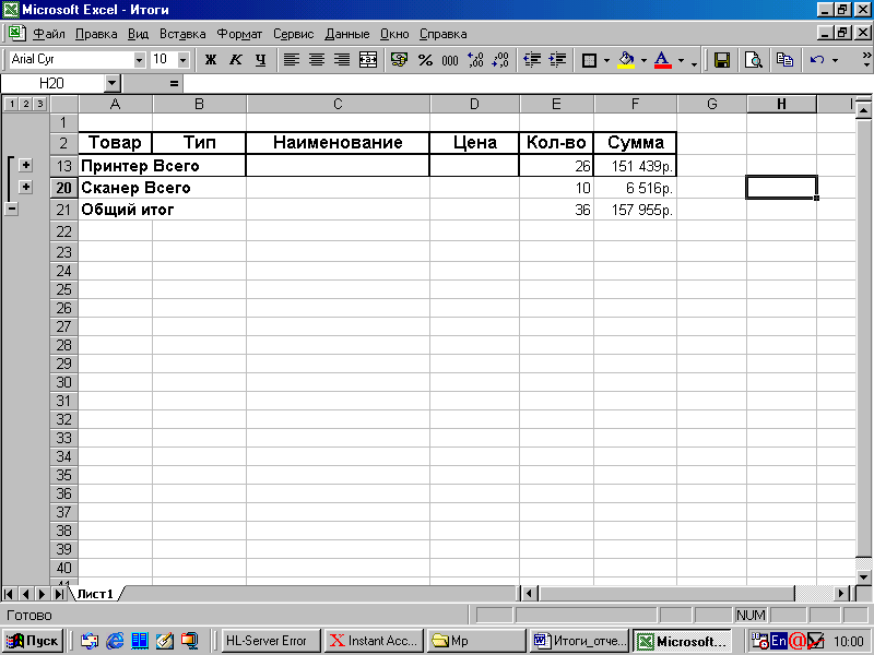
Fig. 5. Option for displaying totals.
To delete entered subtotals, just select the command Outcome on the menu Data and click the button Remove all .
Calculate yourself :
Average price of printers and scanners;
The number of varieties of names of printers and scanners;
Amounts spent on the purchase of each type of product (Fig. 6)
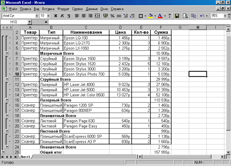 Fig. 6. Amounts spent on the purchase of each type of product.
By default, rows containing total values \u200b\u200bwill be inserted below the rows with individual data group values. If totals are to be presented before group data, the option should be disabled. Outcome under the data in the dialog Subtotals .
When printing, each group of data with totals can be presented on a separate page. To do this, set the option End of page between groups in a dialog Subtotals .
Preparation of consolidated reports
The purpose of the assignment: learn how to draw up consolidated reports.
Consolidation function is used when you need to calculate totals for data located in different areas of the table. By using the consolidation function, you can perform the same operations on values \u200b\u200bin non-contiguous ranges of cells as with the automatic subtotal function. The ranges of cells to be consolidated can be located on the same worksheet or on different sheets, as well as in different workbooks.
We will use the previous example as an example. Separate only printer data and scanner data into two workers sheet, rename “ Sheet1”To“ Printers ”and“ Sheet2" in " Scanners”.
We will compile a consolidated report on the purchases of printers and scanners (data placed on different sheets of the workbook). For this:
Select “ Sheet3"And give it a new name" Report”. Create a “header” for the new table (Fig.8);
Select a cell A 7 (“Product”), And in the menu Data select team Consolidation . In the dialog box of the same name that opens, specify the ranges of cells to be consolidated and the type of operation (function) (Fig. 7.):
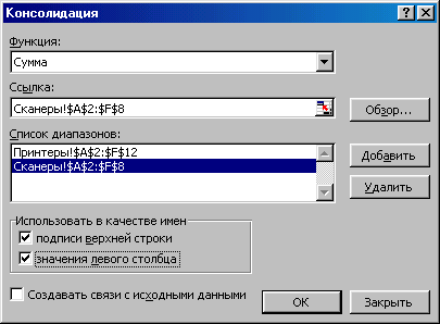
Fig. 7. Dialog window Consolidation
make sure in the box Function is the function Amount ,
click in the box Link and then on the sheet tab “ Printers”, Select the block of cells with information about printers, including the title, click on the button Add to . Follow the same steps with the data for scanners.
set in box Use as names options Top line captions and Left column values to set consolidation by name, and the values \u200b\u200bin rows with the same labels, even if they are located in non-contiguous ranges of cells, will be summed,
Click OK , in the resulting consolidated report the columns “ A type” and “ Name” can be hidden (Fig. 8)
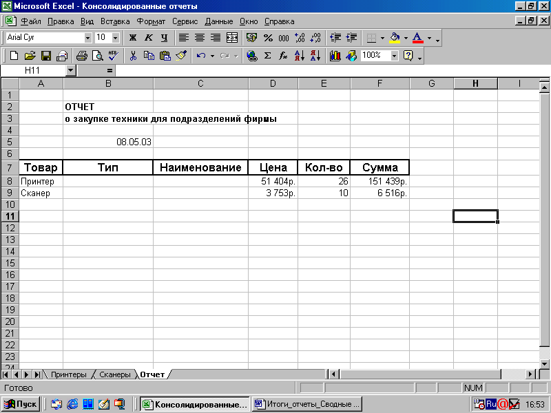
Fig. 8. Consolidated report
If you change the values \u200b\u200bin the original cell ranges, the consolidation must be repeated. If the structure of the source tables (cell ranges) does not change, then the constant repetition of this procedure can be avoided by linking the consolidated data with the original. In this case, the consolidated range of cells will contain cells with external references to the original data. When the data in the original range of cells changes, the consolidated data will also automatically change. To establish links between the consolidated and the original data, set the option Create links to source data in the dialog Consolidation (Fig. 7) .
In this case, after pressing the button OK a dynamic drop will be set between the original data and the consolidation results, ensuring that the data is automatically updated. Consolidation with linking has another advantage: in this case, the data is consolidated using the structuring function, and the second level of the structure presents the individual values \u200b\u200bfrom which the consolidated values \u200b\u200bare calculated.
If the original data is within the same workbook, the update will occur automatically. But for the original data located in other workbooks, the data update will have to be forced using the command Connections menu Edit .
Building pivot tables and pivot charts
Pivot tables are designed for analyzing large amounts of data. With their help, the data of the analyzed table can be selectively presented in a form that best reflects the dependencies between them.
The pivot table is used to analyze the data saved in Excel, that is, for work we need the data that we propose to copy from the following table in Fig. 9 to our worksheet.

Fig. 9. Data for a pivot table.
Create a pivot table.
Select Team Pivot table menu Data or click on the button Pivot tables toolbar to launch the PivotTable and Chart Wizard. A dialog box appears on the screen PivotTable Wizards (Fig. 10) .

Figure: 10 PivotTable Wizard.
In Group Create a table based on the data located : Select the radio button corresponding to the available data sources. In our example, the data is presented in a Microsoft Excel list.
In Group The type of the generated report: install pivot table. Click on the button Further - a window will appear:
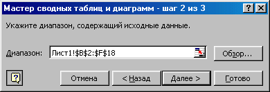
In field Range : (Fig. 11) Specify the range containing the original data. There are two ways to do this: enter the address or name of a range of cells using the keyboard, or select a range of cells in a worksheet using the mouse.

Select the location of the created pivot table (Fig. 12). If you chose a location on the same sheet, specify a location range or just a starting cell.
Click the button Layout…. The dialog box for building a pivot table will appear (Fig. 13).
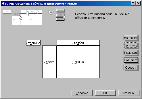
When marking up the layout, drag with the mouse the field buttons in the area:
Drag button Name to the region Line , button Manufacturer to the region Page , button Quarter to the region Column , buttons Turnoverand amount to the region Data (Fig. 14).
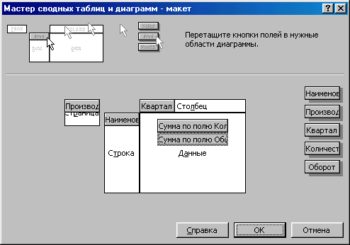
Click the button OK , and then Done ... You will receive a pivot table (Fig. 15.)

Fig. 15 Summary table.
Configuring pivot table options.
Right-click on any cell of the already created PivotTable and from the menu that appears, select Table parameters. A window will appear on the screen Pivot table options (Fig. 16).

Fig. 16. Pivot table parameters window.
In this dialog in the box Name the name of the pivot table is set. Checked boxes Total by columns and Total by lines aboutmeans that the pivot table will be printed Grand total and Field totals... Checked box AutoFormat means the default will be applied to the pivot table AutoFormat... Checked box Include hidden values means that the values \u200b\u200bof the hidden cells will be taken into account in the totals. To combine cells with captions of all outer rows and columns need to check the box Combine header cells ... To protect the cell formats of the pivot table from changes when it is refreshed or the layout is changed, select the checkbox Keep formatting ... In the fields For errors display , For empty cells, display enter the values \u200b\u200bto be displayed in cells in case of error or missing data. These fields will only be available if the corresponding checkboxes are present. Check the box Save data along with a table to copy the original data from which it was created this tableto always have access to them. Check the box Deployment allowed to be able to display detailed data by double-clicking the data area of \u200b\u200bthe pivot table. Check the box Refresh at opening to have the PivotTable refresh when you open the Excel workbook that contains it. In the case of using external sources when creating a pivot table, set the necessary parameters in the group External data .
Close the window by clicking the button OK .
Filtering data.

Click OK , additional sheets have appeared in your workbook. Excel will put each group of data on a separate worksheet.
Detailed data display.
Double-click the field element for which you want to display details. A window will appear on the screen Show details (Fig. 18).

Fig. 18. Window for displaying detailed data.
Select the field containing the parts you want to show from the list provided and click the button OK ... The corresponding rows or columns are inserted into the pivot table.

Fig. 19. Detailed pivot table data.
To not display the detailed data, double-click the data field item again.
Sorting data.
The fields in the pivot table are automatically sorted in ascending order according to their names; you can change the sort order later.
Sort data by field Grand total... To do this, select the data for sorting, select from the menu Data element Sorting ... A dialog box appears on the screen Sorting ... Set the range in the group Sort by , and in the group Sort set the switch meaning ... Click the button OK (Fig. 20).

Fig. 20 Data sorting window.
To automatically sort the data fields by name when updating (changing) the table, double-click the button of the field to be sorted and in the window that appears click on the button Further ... A window will appear on the screen (Fig. 21). In Group Sorting options set the radio button in ascending or descending order, in the list using the field, select the field whose elements will be sorted. Close the window.
![]()
Fig. 21. Additional parameters window.
To manually sort the PivotTable items by data area cell values, in the dialog Additional pivot table field options in Group Sorting options set the switch manually , then close the window. Select the field to sort and choose the command Sorting menu Data . In the window that appears in the field sort by specify the field of the data area to be sorted. Start sorting. If the pivot table contains items that are usually not sorted alphabetically but chronologically, such as Sunday, Monday, Tuesday, etc. Excel automatically uses a custom sort order. Excel contains multiple sort lists, and using the tab Lists window Options (element Options menu Service ) you can define your own sorting list.
Display of the '' top ten '' data.
In the created pivot table, you can reflect the specified number of items only with the maximum or minimum values.
Double-click on the data field whose items will be selectively displayed.
In the window that appears Calculating a PivotTable Field click on the button Further ... A window will appear on the screen Additional pivot table field options .
In Group Display options set the switch automatic(Fig. 21). In field display specify the number of displayed items, and in the list display select the desired sorting option: the greatest or the smallest ... In the list using the fieldselect the data field whose items will be displayed. Click on the button OK ... Close the window.
Changing the function for calculating grand totals.
When you create a PivotTable, Excel automatically displays grand totals, using the sum function to calculate in fields with numeric values \u200b\u200band a function to count the number of values \u200b\u200bin fields with other data. These functions can be changed later.
Click on the button Field parameters on the toolbar Pivot tables ... A window will appear on the screen Pivot table field calculation.
Select a suitable function from the list Operation (Fig. 22) and click the button OK .
![]()
Fig. 22. Application of functions for calculating grand totals.
Specifying additional calculations when summing up.
You can also use another group of functions to summarize, which allows you to calculate the totals of values \u200b\u200bin a data area based on other values \u200b\u200bin a data area in order to compare them.
Select the field in the pivot table that contains the automatically summarized table.
Click on the button Field parameters on the toolbar Pivot tables . A window will appear on the screen Calculating a PivotTable Field ... Click on the button Additionally , to expand the window.
Select from the list Additional calculations desired function. If necessary in the list field select the field name, and in the list element - an element used as a base value when performing additional calculations. Click on the button OK (Fig. 23.)

Fig. 23. Performing additional calculations.