All the same a certain amount. Examples of using the summed function in excel

To sum the values \u200b\u200bthat meet the specified criterion (condition), use the SUMIF () function , English version SUMIF ().

Function syntax

SUMIF(Range; Condition; [Sum_range])

Range - the range of cells in which the values \u200b\u200bcorresponding to the argument are searched Condition... The range can contain numbers, dates, text values, or references to other cells. In case the other argument is Sum_range - is omitted, then the argument Range is also the range over which the sum of values \u200b\u200bsatisfying the argument is performed Condition (in this case Range must contain numbers).

Condition - a criterion in the form of a number, expression or text that determines which cells should be added. For example, the argument Condition can be expressed as 32, "apples" or "\u003e 32".

Sum_range - a range of cells containing numbers that will be summed if the corresponding cells specified in the argument Rangematch the argument Condition. Sum_range - optional argument. If it is omitted, then the sum will be performed over the range of cells specified in the argument Range.

Examples of

Consider the case where the argument Sum_range omitted. In this case, the sum will be performed over the range of cells specified in the first argument Range (i.e. it must contain numbers). It will also search for values \u200b\u200bcorresponding to the argument Condition, which will then be summed up. Let it be a range B5: B15 , see example file.

We will solve the problems:

find the sum of all numbers greater than or equal to 10. Answer: 175. Formula: \u003d SUMIF (B5: B15, "\u003e \u003d 10")
find the sum of all numbers less than or equal to 10. Answer: 42. Formula: \u003d SUMIF (B5: B15, "<=10")
find the sum of all positive numbers in a range. Formula: \u003d SUMIF (B5: B15, "\u003e 0")... An alternative version using the SUMPRODUCT () function looks like this: \u003d SUMPRODUCT ((B5: B15) * (B5: B15\u003e 0))

Task form terms(criterion) is flexible enough. For example, in the formula \u003d SUMIF (B5: B15; D7 & D8) criterion<=56 задан через ссылку D7&D8 : в D7 contains text value<=, а в D8 - number 56 (see figure below). The user, for example, can easily change the criterion using in the cell D7 ... Equivalent formula \u003d SUMIF (B5: B15, "<=56") или \u003d SUMIF (B5: B15, "<="&56) or \u003d SUMIF (B5: B15, "<="&D8) or \u003d SUMIF (B5: B15; D7 & 56).

The SUMIF function is used when you need to sum the values \u200b\u200bin a range that meet a specified criterion.

Function description

The SUMIF function is used when you need to sum the values \u200b\u200bin a range that meet a specified criterion. For example, in a column of numbers, you only need to add up values \u200b\u200bgreater than 5. To do this, you can use the following formula:
\u003d SUMIF (B2: B25, "\u003e 5") In this example, the summed values \u200b\u200bare checked against the criterion. If necessary, the condition can be applied to one range, and the corresponding values \u200b\u200bfrom another range can be summed. For example, the formula:
\u003d SUMIF (B2: B5; "Ivan"; C2: C5) sums only those values \u200b\u200bfrom the range C2: C5 for which the corresponding values \u200b\u200bfrom the range B2: B5 are equal to “Ivan”.
Another example of using the function is shown in the figure below:

An example of using SUMIF to calculate profits with a condition

Syntax

\u003d SUMIF (range, condition, [sum_range])

Arguments

range condition sum_range

Required argument. The range of cells to be judged by the criteria. The cells in each range must contain numbers, names, arrays, or number references. Blank cells and cells containing text values \u200b\u200bare skipped.

Required argument. A condition in the form of a number, expression, cell reference, text, or function that determines which cells to sum. For example, a condition can be represented as: 32, “\u003e 32”, B5, “32”, “apples”, or TODAY ().

Important! All text conditions and conditions with logical and mathematical signs must be enclosed in double quotation marks (“). If the condition is a number, you do not need to use quotation marks.

Optional argument. Cells from which values \u200b\u200bare added if they differ from the cells specified as a range. If sum_range is omitted, Microsoft Excel sums the cells specified in the range argument (the same cells that the condition applies to).

Remarks

You can use wildcards in the condition argument: question mark (?) And asterisk (*). The question mark matches any single character, and the asterisk matches any sequence of characters. If you want to find a question mark (or an asterisk) directly, you must put a tilde (~) in front of it.
The SUMIF function returns incorrect results if it is used to match strings longer than 255 characters to the #VALUE! String.
The sum_range argument may not be the same size as the range argument. When determining the actual cells to be totaled, the top-left cell of the sum_range argument is used as the starting cell, and then the cells in the portion of the range that are sized by the range argument are summed.

Let's add the values \u200b\u200bin the rows, the fields of which satisfy two criteria at once (Condition AND). Consider Text criteria, Numeric and Date criteria. Let's analyze the SUMIFS function ( ), English version SUMIFS ().

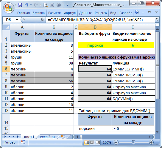
Let's take a table with two columns (fields) as a source table: text " Fruit"And numeric" Quantity in stock"(See example file).

Problem1 (1 text criterion and 1 numeric)

Let's find the number of boxes of goods with a certain Fruit AND, which Remaining boxes in stock not less than the minimum. For example, the number of boxes with goods peaches (cell D 2 ), which have the remaining boxes in the warehouse\u003e \u003d 6 (cell E 2 ) ... We should get the result 64. Counting can be implemented by many formulas, we will give several (see the example file Sheet Text and Number):

1. =SUMIFS (B2: B13; A2: A13; D2; B2: B13; "\u003e \u003d" & E2)

Function syntax: SUMIFS (sum_interval; condition_interval1; condition1; condition_interval2; condition2 ...)

B2: B13 Sum_Interval - cells for summation, including names, arrays or references containing numbers. Empty values \u200b\u200band text are ignored.
A2: A13and B2: B13 condition_interval1; condition_interval2; ... represent from 1 to 127 ranges in which the corresponding condition is checked.
D2and "\u003e \u003d" & E2 Condition1; condition2; ... are from 1 to 127 conditions in the form of a number, expression, cell reference or text, which determine which cells will be summed.

The order of the arguments is different in the SUMIF () and SUMIF () functions. The SUMIFS () argument summation_interval is the first argument, and in SUMIF () the third. When copying and editing these similar functions, make sure that the arguments are in the correct order.

2.other option \u003d SUMPRODUCT ((A2: A13 \u003d D2) * (B2: B13); - (B2: B13\u003e \u003d E2))
Let's take a closer look at using the SUMPRODUCT () function:

The result of evaluating A2: A13 \u003d D2 is an array (FALSE: FALSE: FALSE: FALSE: TRUE: TRUE: TRUE: FALSE: FALSE: FALSE: FALSE: FALSE) The TRUE value matches the value from the column AND criterion, i.e. word peaches... The array can be seen by highlighting in A2: A13 \u003d D2 and then pressing;
The result of calculating B2: B13 is (3: 5: 11: 98: 4: 8: 56: 2: 4: 6: 10: 11), i.e. just values \u200b\u200bfrom a column B ;
The result of elementwise multiplication of arrays (A2: A13 \u003d D2) * (B2: B13) is (0: 0: 0: 0: 4: 8: 56: 0: 0: 0: 0: 0). Multiplying a number by FALSE results in 0; and for the value TRUE (\u003d 1) the number itself is obtained;
Let's analyze the second condition: The result of the calculation - (B2: B13\u003e \u003d E2) is an array (0: 0: 1: 1: 0: 1: 1: 0: 0: 1: 1: 1). The values \u200b\u200bin the column " Number of boxes in stock»That meet the criterion\u003e \u003d E2 (ie\u003e \u003d 6) correspond to 1;
Further, the SUMPRODUCT () function multiplies the elements of the arrays in pairs and sums the resulting products. We get - 64.

3. Another use of the SUMPRODUCT () function is the formula \u003d SUMPRODUCT ((A2: A13 \u003d D2) * (B2: B13) * (B2: B13\u003e \u003d E2)).

If necessary, dates can be entered directly into the formula \u003d SUMIFS (B6: B17; A6: A17; "\u003e \u003d 01/15/2010"; A6: A17; "<=06.03.2010")

To display the selection criteria in a text string, use the formula \u003d "Sales volume for the period from" & TEXT (D6; "dd.MM.yy") & "to" & TEXT (E6; "dd.MM.yy")

Used in the last formula.

Task4 (Month)

We slightly modify the condition of the previous problem: find the total sales for the month (see the example file Sheet Month).

Formulas are constructed similarly to task 3, but the user enters not 2 dates, but the name of the month (it is assumed that the data in the table is within 1 year).

To solve the 3rd task, the table with the configured autofilter looks like this (see the example file Sheet 2 Dates).

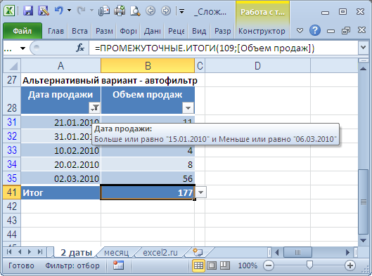
Previously, the table must be converted to and include the Totals row.

Good afternoon, dear subscribers and visitors of the blog site. Quite recently, we figured out the VLOOKUP formula, and immediately afterwards I decided to write about another very useful Excel function - SUMIF... Both of these functions are able to "link" data from different sources (tables) by key field and under some conditions are interchangeable. At the same time, there are significant differences in their purpose and use.

If the purpose of VLOOKUP is simply to "pull" data from one place in Excel to another, then SUMIF is used to sum up the numerical data according to a given criterion. The main purpose of this formula is to summarize data in accordance with some condition. Something like this is written in the help. However, this tool will work for other purposes as well. For example, I often use the SUMIF formula instead of VLOOKUP, since it does not generate # N / A errors when it cannot find something. And this greatly facilitates and speeds up the work.

The SUMIF function can be successfully adapted to solve a wide variety of problems. Therefore, in this article, we will consider not 1 (one), but 2 (two) examples. The first one will be associated with summation according to a given criterion, the second - with data “pulling”, that is, as an alternative to VLOOKUP.

Example of Summing Using the SUMIF Function

The table contains positions, their quantities, as well as belonging to a particular group of goods (first column). Consider for now a simplified use of SUMIF, when we need to calculate the amount only for those positions, the values \u200b\u200bfor which correspond to a certain condition. For example, we want to know how many top positions were sold, i.e. those whose value exceeds 70 units. It is not very convenient and fast to search for such goods with your eyes, and then summarize manually, therefore the SUMIF function is very appropriate here.

First of all, select the cell where the amount will be calculated. Next, we call the Function Wizard. This is the icon fx on the formula bar. Next, look for the SUMIF function in the list and click on it. A dialog box opens, where, to solve this particular problem, you need to fill in only two (first) fields out of the three proposed.

That is why I called this example simplified. Why 2 (two) out of 3 (three)? Because our criterion is in the very range of summation.

The "Range" field indicates the area of \u200b\u200bthe Excel table where all the original values \u200b\u200bare located, from which you need to select something and then add. It is usually set with the mouse.

The "Criterion" field indicates the condition by which the formula will select. In our case, we indicate "\u003e 70". If you do not put the quotes, then they will be completed by themselves. But in general, such a criterion should be in quotation marks.

We do not fill in the last field "Sum_range", since it is already indicated in the first field.

Thus, the SUMIF function takes a criterion and begins to select all values \u200b\u200bfrom the specified range that meet the specified criterion. After that, all the selected values \u200b\u200bare added. This is how the function algorithm works.

Having filled in the required fields in the Function Wizard, press the big "Enter" button on the keyboard, or click on "OK" in the Wizard window. After this, the calculated value should appear at the place of the input function. In my example, it turned out 224pcs. That is, the total value of goods sold in the amount of more than 70 pieces was 224 pieces. (this can be seen in the lower left corner of the Wizard window even before clicking "ok"). That's all. This was a simplified example where the criterion and the summation range are in the same place.

Now let's look at an example where the criterion does not match the summation range. This situation is much more common. Consider the same conditional data. Suppose we need to know the amount no more or less than some value, but the amount of a specific group of goods, for example, group G.

To do this, again select the cell with the future calculation of the amount and call the Function Wizard. Now, in the first window, we indicate the range that contains the criterion by which the selection will be made for summing, that is, in our case, this is a column with the names of product groups. Further, the criterion itself is prescribed either manually, leaving the entry "group D" in the appropriate field, or simply indicate with the mouse the cell with the required criterion. The last box is the range where the summarized data is located. We indicate it with the mouse, but lovers of printing are not prohibited from typing manually.

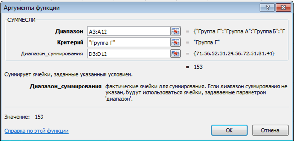
The result will be the amount of goods sold from group D - 153 pcs.

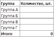
So, we looked at how to calculate one amount for one specific criterion. However, more often the problem arises when it is required to calculate several amounts for several criteria. It couldn't be easier! For example, we need to find out the amount of products sold for each group. That is, I am interested in 4 (four) values \u200b\u200bfor 4 (four) groups (A, B, C and D). For this, a list of groups is usually made somewhere in the open spaces of Excel in the form of a separate table. It is clear that the names of the groups must exactly match the names of the groups in the source table. Let's immediately add the final line, where the sum is still zero.

Then the formula for the first group is prescribed and extended to all the others. Here you just need to pay attention to the relativity of links. The range with the criteria and the summation range should be absolute links, so that when you drag the formula, they do not "go down", but the criterion itself, firstly, you need to specify with the mouse (and not manually write), and secondly, it should be a relative link, so how each sum has its own summation criterion.

The filled-in fields of the Function Wizard with such a calculation will look something like this.

As you can see, for the first group A, the amount of goods sold was 161 pieces (lower left corner of the figure). Now press enter and drag the formula down.

All amounts were calculated, and their grand total is 535, which coincides with the total in the original data. This means that all values \u200b\u200bhave been summed up, nothing has been missed. The last use case for SUMIF personally occurs to me quite often.

An example of using the SUMIF function to compare data

As I've noted more than once, the SUMIF function can be used sensibly to bind data. Indeed, if you add up one value, you get that value itself. This arithmetic property is not a sin to use for good. It is even possible that the designers of Excel are not aware of such barbaric use of their brainchild.

In short, SUMIF is easy to adapt for data binding as an alternative to VLOOKUP. Why use SUMIF when VLOOKUP exists? Let me explain. First, SUMIF, unlike VLOOKUP, is insensitive to the data format and does not generate an error where you least expect it; secondly, SUMIF instead of errors due to the lack of values \u200b\u200baccording to a given criterion gives 0 (zero), which allows you to calculate the totals of the range with the SUMIF formula without unnecessary gestures. However, there is one drawback. If any criterion is repeated in the desired table, then the corresponding values \u200b\u200bwill be summed up, which is not always a "pull-up". Better to be on your guard. On the other hand, this is often necessary - to pull up the values \u200b\u200bto a given place, and at the same time add the duplicated positions. You just need to know the properties of the SUMIF function and use it according to the instruction manual.

Now let's look at an example of how the SUMIF function turns out to be more suitable for pulling data than VLOOKUP. Let the data from your example be the sales of some products in January. We want to know how they changed in February. It is convenient to make a comparison in the same plate, having previously added one more column to the right and filled it with data for February. Somewhere in another Excel file there is statistics for February for the entire assortment, but we want to analyze exactly these positions, for which we need to pull up the necessary values \u200b\u200bfrom a large file with sales statistics for all products into our table. First, let's try using the VLOOKUP formula. We will use the product code as a criterion. The result is in the figure.

It is clearly seen that one position has not been tightened, and the # N / A error is displayed instead of a numerical value. Most likely, this product was simply not on sale in February, and therefore it is missing from the February database. As a result, the # N / A error is shown in total. If there are not many positions, then the problem is not big, it is enough to manually remove the error and the amount will be recalculated correctly. However, the number of lines can be measured in hundreds, and counting on manual adjustments is not quite the right decision. Now let's use the SUMIF formula instead of VLOOKUP.

The result is the same, only instead of the # N / A SUMIF error it gives zero, which allows you to normally calculate the amount (or another indicator, for example, the average) in the final row. This is the main idea why SUMIF should sometimes be used instead of VLOOKUP. With a large number of positions, the effect will be even more noticeable.

In reality, it is often necessary to work with large amounts of data that are many times larger than the size of the monitor. It is very difficult to spot and track errors. But all the jambs pop up in subsequent calculations. It is not convenient to disassemble such examples using the screenshots in the article, so I invite you to watch a specially recorded video tutorial about the SUMIF function.

Here's another lesson on SUMIF