How to put the formula for adding cells in Excel. How to calculate the amount in Excel in different ways?

Adds values. You can add single values, ranges of cells, cell references, or all three of these kinds of data.

\u003d SUM (A2: A10)

\u003d SUM (A2: A10; C2: C10)

This video is part training course Add numbers in Excel 2013.

Syntax

SUM (number1; [number2]; ...)

Quick summation in the status bar

If you need to quickly get the sum of a range of cells, you just need to select the range and look at the lower right corner of the Excel window.

Status bar

The information in the status bar depends on the current selection, whether it is one cell or several. If you right-click on the status bar, a pop-up dialog box appears with all the available options. If you select any of them, the corresponding values \u200b\u200bfor the selected range appear in the status bar. Learn more about the status bar.

Using the AutoSum Wizard

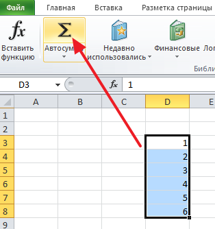
The easiest way to add the SUM formula to a sheet is by using the AutoSum Wizard. Select a blank cell directly above or below the range you want to sum, and then open the Home or Formula tab on the ribbon and click AutoSum\u003e Sum... The Auto Sum Wizard automatically determines the range to sum and generates a formula. It can also work horizontally if you select a cell to the right or left of the range to be summed, but this will be covered in the next section.

Quickly Add Adjacent Ranges with the AutoSum Wizard

You can also select other standard functions in the AutoSum dialog box, for example:

Auto-sum vertical

The AutoSum Wizard automatically identifies cells B2: B5 as the range to total. You only need to press Enter to confirm. If you need to add or exclude multiple cells, hold down the SHIFT key, press the appropriate arrow key until you select the range you want, and then press Enter.

Intellisense hint for the function. The floating tag SUM (number1; [number2];…) below the function is an Intellisense hint. If you click SUM or another function name, it changes to a blue hyperlink that takes you to the Help topic for that function. As you click individual elements of a function, the corresponding portions in the formula will be highlighted. In this case, only cells B2: B5 will be selected because there is only one numeric reference in this formula. The Intellisense tag appears for any function.

Horizontal AutoSum

Using the SUM function with continuous cells

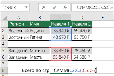
The AutoSum wizard usually only works on contiguous ranges, so if your range to sum contains empty rows or columns, Excel will stop at the first skip. In this case, you need to use the SUM function by selection, in which you add individual ranges sequentially. In this example, if you have data in cell B4, Excel will create the formula \u003d SUM (C2: C6) because it recognizes a contiguous range.

To quickly select multiple non-contiguous ranges, press CTRL + left click... First enter "\u003d SUM (", then select different ranges, and Excel will automatically add a semicolon between them as a separator. When finished, press Enter.

ADVICE. You can quickly add the SUM function to a cell using the keys ALT + \u003d... After that, you just have to select the ranges.

Note.You may have noticed that Excel colorizes different ranges of function data and the corresponding fragments in the formula: cells C2: C3 are highlighted in one color, and cells C5: C6 in another. Excel does this for all functions, unless the referenced range is in another sheet or workbook. To use accessibility more efficiently, you can create named ranges, such as Week1, Week2, and so on, and then refer to them in a formula:

\u003d SUM (Week1; Week2)

Add, subtract, multiply and divide in Excel

Excel makes it easy to perform mathematical operations, either individually or in combination with excel functions, for example SUM. The table below lists the operators that you might find useful, as well as their associated functions. Operators can be entered either using the numeric row on the keyboard, or using the numeric keypad, if you have one. For example, using the Shift + 8 keys, you can enter an asterisk (*) to multiply.

For more information, see Use Microsoft Excel as a Calculator.

Other examples

Perhaps one of the most popular functions of the program Microsoft Excel is addition. The ease of working with Excel in summing values \u200b\u200bmakes a calculator or other ways to add large arrays of values \u200b\u200balmost useless. An important feature of addition in Excel is that the program provides several ways to do this.

AutoSum in Excel

The fastest and by far the easiest way to withdraw an amount in Excel is the AutoSum service. To use it, you need to select the cells that contain the values \u200b\u200bthat you want to add, as well as the empty cell immediately below them. In the "Formulas" tab, click on the "AutoSum" sign, after which the result of addition appears in an empty cell.

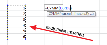
The same method is available in reverse order. In an empty cell, where you want to display the result of addition, you need to put the cursor and click on the "AutoSum" sign. After clicking in a cell, a formula with a free summation range is formed. Using the cursor, select a range of cells, the values \u200b\u200bof which need to be added, and then press Enter.

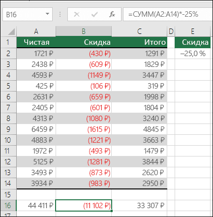
Cells for addition can also be defined without selection with the cursor. The formula for the sum is: "\u003d SUM (B2: B14)", where the first and last cells of the range are given in brackets. By changing the values \u200b\u200bof the cells in the Excel table, you can adjust the summation range.

Sum of values \u200b\u200bfor information

Excel not only allows you to sum values \u200b\u200bfor some specific purpose, but also automatically counts the selected cells. Such information can be useful in cases where the task is not related to the summation of numbers, but consists in the need to look at the value of the sum at an intermediate stage. To do this, without resorting to writing a formula, it is enough to select the necessary cells and in the command line of the program at the very bottom of the right-click on the word "Done". In the context menu that opens opposite the "Amount" column, the value of all cells will be displayed.

Simple addition formula in Excel

In cases where the values \u200b\u200bfor addition are scattered throughout the table, you can use a simple addition formula in the Excel table. The formula has the following structure:

To create a formula in a free cell, where the amount should be displayed, put an "equal" sign. Excel automatically responds to this action like a formula. Next, using the mouse, you need to select the cell with the first value, after which the plus sign is placed. Further, all other values \u200b\u200bare also entered into the formula through the addition sign. After the chain of values \u200b\u200bis typed, the Enter button is pressed. The use of this method is justified when adding a small number of numbers.

SUM formula in Excel

Despite the almost automated process of using addition formulas in Excel, it is sometimes easier to write the formula yourself. In any case, their structure must be known in cases where the work is carried out in a document created by another person.

The SUM formula in Excel has the following structure:

SUM (A1; A7; C3)

When typing a formula yourself, it is important to remember that spaces are not allowed in the structure of the formula, and the sequence of characters must be clear.

The sign ";" serves to define a cell, in turn, the ":" sign sets a range of cells.

An important nuance - when calculating the values \u200b\u200bof the entire column, you do not need to set the range, scrolling to the end of the document, which has a border of over 1 million values. It is enough to enter a formula with the following values: \u003d SUM (B: B), where the letters represent the column to be calculated.

Excel also allows you to display the sum of all cells in the document without exception. To do this, the formula must be entered in a new tab. Let's say that all the cells whose sums need to be calculated are located on Sheet1, in which case the formula should be written on Sheet2. The structure itself looks like this:

SUM (Sheet1! 1: 1048576), where the last value is the numerical value of the most recent cell of Sheet1.

Related Videos

An Excel spreadsheet processor is an excellent solution for processing all kinds of data. With it, you can quickly make calculations with regularly changing data. However, Excel is quite a complex program and therefore many users do not even begin to learn it.

In this article, we will show you how to calculate the amount in Excel. We hope this material will help you get familiar with Excel and learn how to use its basic functions.

How to calculate the sum of a column in Excel

Also, the "Auto amount" button is duplicated on the "Formulas" deposit.

After selecting a column with data and clicking on the "Auto Sum" button, Excel will automatically generate a formula for calculating the sum of the column and insert it into the cell immediately below the column with data.

If this arrangement of the column amount does not suit you, then you can specify where you want to place the amount yourself. To do this, you need to select a cell suitable for the amount, click on the "AutoSum" button, and then select the column with the data with the mouse and press the Enter key on the keyboard.

In this case, the column sum will be located not under the data column, but in the table cell you have selected.

How to calculate the sum of specific cells in Excel

If you need to calculate the sum of certain cells in Excel, you can also do this using the "Auto Sum" function. To do this, select with the mouse the cell of the table in which you want to place the amount, click on the "Auto amount" button and select the required cells while holding down the CTRL key on the keyboard. After the required cells are selected, press the Enter key on the keyboard, and the amount will be placed in the cell of the table you have selected.

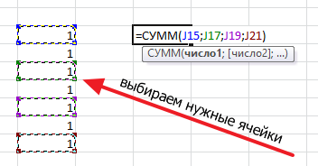
In addition, you can enter a formula to calculate the sum of certain cells manually. To do this, place the cursor where the amount should be, and then enter the formula in the format: \u003d SUM (D3; D5; D7). Where instead of D3, D5 and D7 are the addresses of the cells you need. Please note that cell addresses are entered separated by commas, no comma is needed after the last cell. After entering the formula, press the Eneter key and the amount will appear in the cell you selected.

If the formula needs to be edited, for example, you need to change the addresses of the cells, then for this you need to select the cell with the amount and change the formula in the row for the formulas.

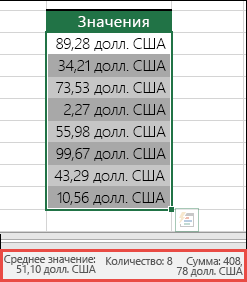
How to quickly view the amount in Excel

If you need to quickly see what amount will turn out if you add certain cells, and at the same time you do not need to display the value of the amount in a table, then you can simply select the cells and look down the Excel window. There you can find information about the sum of the selected cells.

It will also show the number of selected cells and their average value.

The most simple formula in Excel, it is perhaps the sum of the values \u200b\u200bof certain cells.

The simplest example: you have a column of numbers, the sum of these numbers must be below it.

Select cells with values, and another empty one below them, where the value of the sum should be located. And click on the autosum button.

Another option is to mark the cell where the value of the sum should be, press the autosum button.

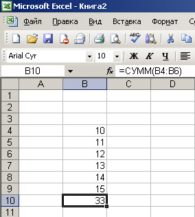
the area, the values \u200b\u200bof which will be summed up, is highlighted and in the sum cells we see the range of the summed cells. If the range is what you want, just press Enter. The range of the summing cells can be changed

For example B4: B9 can be replaced with B4: B6 see.

and we will get the result

Now let's look at a more complex option.

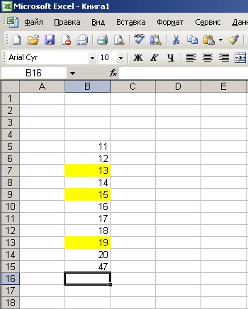
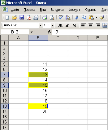
Let's say you need to add the values \u200b\u200bof cells that do not stand in a row in a row, one below the other. In the figure, cells are highlighted in yellow, the values \u200b\u200bof which we will add.

We put the cursor on the cell where the sum of the yellow cells should be. We press the "equal" sign, then we press on the first yellow cell, and the formula begins to form in our cell of the sum. Then we press the plus sign (+), after it we press the next yellow cell, then again the plus, and the last yellow cell, we see the following on the screen:

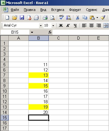
It happens that you are not faced with the task of a specific cell was the value of the sum of cells. Let's say you need to quickly see how many values \u200b\u200bmake up the sum. In Excel, this is possible.

Let's use the old example with yellow cells.

There is a status bar at the bottom of the sheet. Now it says “Done”.

If you right-click, a menu will appear, in it we select the value "amount"

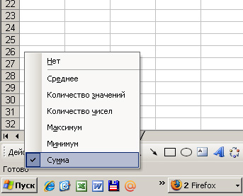
Notice that the value of the sum of yellow cells appears in the lower right corner.

- a program for creating tables, which is widely used both in organizations and at home, for example, for home bookkeeping. During using Excel many users are faced with the fact that it is necessary to calculate the sum of a column. Of course, you can do it manually, but it's much easier to follow the advice given in the article.

Below we will look at several ways to help you get the sum of cells in a column.

Today we will look at:

Method 1

Just select the cells with the mouse and then click the autosum icon. The total will be displayed in an empty cell below.

Method 2

Another variant. Click on the empty cell where the amount should be displayed, and then click on the autosum icon.

The program will highlight the area to be added, and the formula will be displayed in the place where the total will be located.

You can easily adjust this formula by changing the values \u200b\u200bin the cells. For example, we need to calculate the amount not from B4 to B9, but from B4 to B6. When you finish typing, press the Enter key.

Method 3

But what if the cells required for the summation are not one after another, but scattered? This task is a little more difficult, but it is also easy to cope with it.

For clarity, the cells that we need to fold, we will highlight with color. Now click with the mouse cursor on the cell where the amount will be located and put the sign = ... It is with such a sign that any formula begins.

Now click on the first cell to be summarized. In our case, this is B7. The cell appears in the formula. Now put a sign + and add the rest of the cells in the same way. You will get something like the screenshot below.

Press Enter to execute the formula. The system will display the number with the sum of the cells.