How to change the date in the Excel table. How to insert a static, fixed, non-updatable date into a cell? Select from a list of date formats.
The format of a cell in Excel is not easy to define appearance displaying data, but also tells the program itself exactly how it should be processed: as text, as numbers, as a date, etc. Therefore, it is very important to correctly set this characteristic of the range in which the data will be entered. Otherwise, all calculations will simply be incorrect. Let's find out how to change the format of cells in Microsoft Excel.
If you want to edit the contents of a cell, you usually turn to the mouse and the cursor will move to the desired position in the cell by double-clicking on it. You can now adapt the content accordingly or enter a value. But it's easier to do this without choosing the "long" path over the mouse.
This allows a line break within a cell
The cursor is already active in the cell. This saves you a lot of time when you need to edit an extensive spreadsheet and don't have to constantly use the mouse. Now if you enter text into a cell, you sometimes need a line break. Therefore, move the cursor to the desired transition point.
Switching between tables
In addition, there is a useful keyboard shortcut that you can use to save mouse detour.Let's immediately determine what cell formats exist. The program offers to choose one of the following main types of formatting:
- General;
- Monetary;
- Numerical;
- Financial;
- Text;
- The date;
- Time;
- Fractional;
- Percentage;
- Additional.
In addition, there is a division into smaller structural units of the above options. For example, date and time formats have several subspecies (DD.MM.YY, DD.month.YY, DD.M, H.MM PM, HH.MM, etc.).
In most cases, this is also required in the next bottom cell. For example, if you need to enter a large number of column labels, then the corresponding values \u200b\u200bon the next line. You can take a detour using the arrow key after entering the column heading. Then you need to move your right hand from the block of letters to the arrow keys and then go back. This procedure is, of course, quite adequate. It is even more impractical to grab after the mouse to get to the desired next cell.
Fill multiple cells with the same content

But it's even easier without changing the settings in the Options section. Now it may happen that you need to fill several cells with the same content in the table. Just run cell for cell and enter your desired content. The offer is black. If you agree with this proposal, just press the "Enter" button and it is already accepted. This makes the job much easier.
There are several ways to change the formatting of cells in Excel. We will talk about them in detail below.
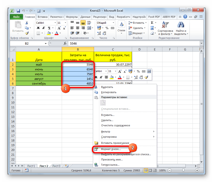
Method 1: context menu
The most popular way to change data range formats is by using the context menu.
Show formulas back
But there are more effective method get to the finish line. Especially if you need to fill many cells with the same content. 
For these formulas to be visible, you need to click on the corresponding cell and the edited formula will be displayed in the processing line.
Show all formulas at the same time
Or double-click in the cell and instead of the value displayed by the formula. This is often the case that no one knows at all what meaning the formula has. It is cumbersome to check all cells with a value to check if the value is the result of a formula.
After these steps, the format of the cells is changed.
Method 2: toolbox "Number" on the ribbon
Formatting can also be changed using the tools found on the ribbon. This method is even faster than the previous one.


Thus, from Arabic Roman numerals
But there is a little trick or, better, a keyboard shortcut that displays all the stored formulas in a table. Click the Show Formula button. Alternatively, you can click the Show Formula button on the Formulas tab. Have you already turned them into your head? 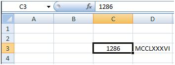
If you've ever tried to get into links, you might have wondered about the results.
The fractional or decimal value is not displayed, but the fraction is converted to a date. We want to enter a fraction and display it. Now there is a little trick on how to deal with this "problem." If you enter 0, then a space, and then a break, the reversal is displayed correctly.
Method 3: toolbox "Cells"
Another option for setting this range characteristic is to use the instrument in the settings block "Cells".

Method 4: hotkeys
Finally, the range formatting window can be invoked using the so-called hot keys. To do this, you must first select the area to be changed on the sheet, and then type the combination on the keyboard Ctrl + 1... After that, a standard formatting window will open. We change the characteristics in the same way as mentioned above.
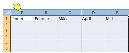
Just adjust the column width
The fraction is displayed in the cell, and the decimal value is displayed in the form bar. So now you can expect a faction. Suppose you have a table with column headings of varying lengths. Now you want to adjust the width of the columns to match the length of the month names.
Same width for multiple columns
The return trip is also possible. Therefore if you have columns of different widths and want to have the same width. When you release the left mouse button, all the selected columns have the same width.
- Select the desired columns as described above.
- Move the mouse pointer over to the right edge of the column until it becomes a cross.
- Use the left mouse button to adjust the column width.
In addition, individual hotkey combinations allow you to change the format of cells after selecting a range, even without calling a special window:
- Ctrl + Shift + - - general format;
- Ctrl + Shift + 1 - numbers with a separator;
- Ctrl + Shift + 2 - time (hours.minutes);
- Ctrl + Shift + 3 - dates (DD.MM.YY);
- Ctrl + Shift + 4 - monetary;
- Ctrl + Shift + 5 - percentage;
- Ctrl + Shift + 6 - OOOE + 00 format.
As you can see, there are several ways to format areas at once. excel worksheet... This procedure can be performed using the tools on the ribbon, calling the formatting window, or hotkeys. Each user decides for himself which option is most convenient for him in solving specific tasks, because in some cases it is enough to use general formats, and in others, an exact indication of characteristics by subspecies is required.
Search multiple tables at the same time
The book consists of several tables. It is now entirely possible that multiple tables are busy with data. And a lot of the data often leads to a limited overview. It can then be tedious to find an accelerated value or formula that you do not know on which sheet of the table you want to search in the book.
But there is a search function. Searching a workbook is pretty straightforward. You don't have to look at every table. Click the Options button. Now you can customize your search parameters. Since we want to search for the entire workbook, not just one table, we need to select the appropriate option.
| lesson 2 | lesson 3 | lesson 4 | lesson 5
Now click "Find All" and you will see a list of search results, from which the table sheet is located and in which cell the found value was found. By the way, you can also use this search to determine where and where to search, for example, to restrict your search to stored formulas.
However, the more such comments accumulate, the more difficult it becomes. Of course, we are not talking about the formulas themselves, but about many comments. The comment is already displayed here because the mouse is on the cell. By changing the parameters, you can make all comments visible at the same time. The result is what the option promised, but it's completely useless here as the following image shows the same file.
I think that from the last lesson you already know that dates and times in Excel are stored in the form of ordinal numbers, the origin of which is considered to be a certain January 0, 1900... Fortunately, in the cells we see not these numbers, but the dates and times that are familiar to us, which can be stored in a variety of formats. In this lesson, you will learn how to enter dates and times in Excel to get the required formatting.
The second option is to print comments. Again, you can make sure all comments are reprinted. In the dialog box, set comments for comments as on a sheet. If comments with the previous option are visible on the sheet, they will appear on the printout. True, it cannot be convincing, because the comments hide all important numbers.
Slightly could be improved by making comments partially transparent. Double clicking on the edge of a comment no longer displays the dialog you are looking for. A selected comment can only display a format dialog by right-clicking on it and from the Comment Popup Menu.
Entering dates and times in Excel
Dates and times in Excel can be entered as an ordinal number or a fraction of a day, but as you yourself understand, this is not very convenient. In addition, with this approach, the cell will have to apply a certain number format each time.
Excel offers several formats for entering temporary data. If you use this format, Excel will automatically convert the entered date (or time) to an ordinal (fraction of a day) and apply the format to the cell Dates (or Time) set by default.
A transparency of only 25% ensures that the data behind the comments is predominantly visible. As you can see in the following figure, this is not a good solution for multiple superimposed comments. Unfortunately there are no comments, although otherwise they behave like drawing objects. You must format each comment separately. To be able to read any comments on the document at any time, an alternative is to print them according to the data on a separate sheet.
In the Page Setup dialog box, select Comments at the end of the sheet. All data and comments should now be read, but you cannot see the cell addresses in the expression in the absence of row and column headers to find the cell that belongs to the comment.
The figure below shows a table of the date and time input options that Excel supports. The left column shows the values \u200b\u200bto be entered into the cell, and the right one shows the conversion result. It should be noted that dates entered without specifying a year are assigned the current year, namely, the one set in the settings of your operating system.
Change all comments on the sheet
Let's start with the simplest problem that you probably missed before: all comments in the current document should be shown transparently. In the sample file, you can create a new module into which you insert the following procedure.
Transparency \u003d 25 Next end. This code edits all comments of the current sheet in a loop and sets its opacity value to 25% for each. If you want to change other properties of the comment, write down the best for the comment and generate the code found in this loop.
These are not all the options that Excel supports. But even these options will be enough for you.
Some of the date display options shown in the right column may differ. It depends on the regional settings and the date and time display format in the operating system settings.
Working with cells in Microsoft Excel that contain a date or time, you have the ability to apply various formatting to them. For example, you can display in a cell only the day of the week, or only the month and year, or only the time.
Copy all comments to another sheet
To do this, select all cells with a comment, and then select the "Delete Comment" entry from the pop-up menu. The second desire was that the content of the comments should be collected and written into the cells of another sheet. There they can be processed at will.
To do this, you need two tabular sheets, namely an active one with comments and a new one with the copied content of comments. Since after inserting a new sheet, the previous active sheet is no longer active, you must also note this in a variable.
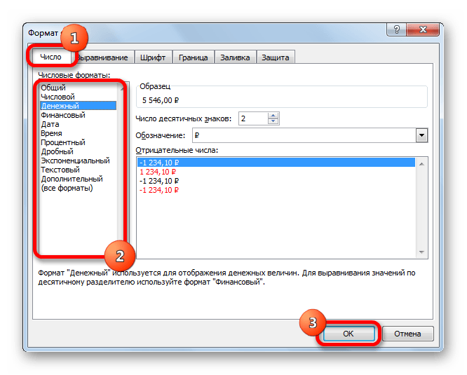
You can get access to all possible formats on the tab Number dialog box Cell format... Category the date the built-in date formats are given:
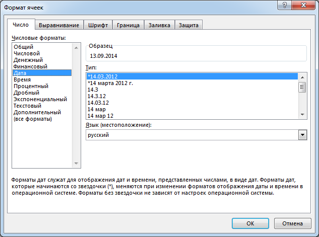
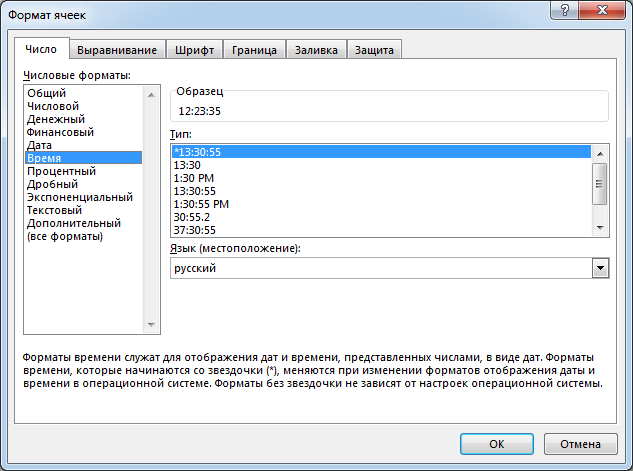
In order to apply formatting to a cell, just select the desired format in the section A type and press OK... The required formatting will be applied. If the built-in number formats are not enough for you, then you can use the category All formats... Here you can also find a lot of interesting things.
Transparency Next end with end sub. For better readability, the code first writes bold to a new sheet. Then all comments are passed and their contents are copied line by line. After a few hand-adjusted column widths and row heights, the result is as follows.
Clearly move comments to the right
Now the best and at the same time the most dangerous macro, because it moves all comments on the sheet to a new position on the right edge. They should be placed so that they do not cover cells with content or other comments. This is an interference with the original comments, which cannot be undone, so the macro always creates a copy of the sheet at the beginning and changes only there.
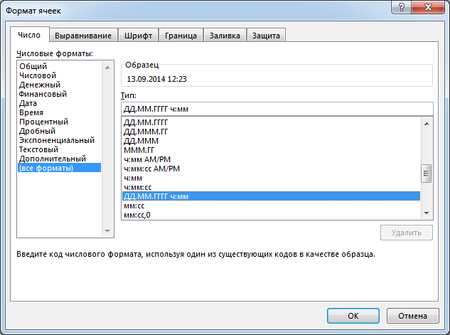
If none of the options suits you, then you can create a custom number format. It's easy enough to create it if you use the built-in number formats as a reference. To create a custom number format, follow these steps:
Opacity \u003d 0 opacity. It is incremented for each comment by its height, as well as by an additional value of 10. As you can see in the following figure, comments are now nicely presented alongside the data. Then, for each comment, its optimal width is set so that it is one line. You don't need to copy all these routines into the comment file.
Many comments can be quite annoying and unwieldy. To provide you with all the content in German, many articles are not translated by humans, but by translation programs that are constantly being optimized. However, machine-translated texts are generally not ideal, especially with regard to grammar and use of foreign words, as well as specialized covers. Microsoft makes no warranty, implied or otherwise, regarding the correctness, correctness, or completeness of the translation.
As you can see, everything is quite simple!
In this lesson, we learned how to customize the format for displaying dates and times in Microsoft Excel, and also discussed several useful options for entering them into a worksheet. In the next lesson, we will talk about 7 Excel functions that allow you to extract the desired parameters from date and time values. This concludes the lesson. All the best and success in learning Excel.